Last year I got an amazing surprise in the mail.
It was an awesome calendar of a handpicked selection of results from the years PlayRaw images.
Chris (@chris) put together another fantastic calendar for this year (while juggling kids, too) and it’s too nice to not have a post about it!
Yep, that’s the back side. Monkey Business by Dimitrios Psychogios (cba)
It was a really awesome surprise to recieve my calendar last year - and I wish I would have planned a little better to be able to grab a photo of the calendar hanging in my office (it’s my work desk calendar - it never fails to remind me that there’s more fun things to life than work - also that I need to up my processing game… ).
This year Chris has done it again by assembling a wonderfully curated collection of images and edits from the various Play Raws that were posted this year.
I’ve plagiarized his post on the forums to put together this post and get some more publicity for his time and effort!
If you get a moment, please thank Chris for his work putting this together!
A preview (also shamelessly lifted from Chris’s forum post):
These Play Raws are a ton of fun and one of the great aspects of having such a generous community to share the images and allowing everyone to practice and play.
I am constantly humbled by the amazing work our community produces and shares with everyone.
Thank you to everyone who shared image and participated in processing (and sharing how you achieved your results)! I have really learned some neat things based on others work and look forward to even more opportunities to play (pun intended).
Fun side note: the Play Raws are actually something that began on the old RawTherapee forums. When they moved their official forums here with us it was one of those awesome things I’m glad they brought over with them (the people were pretty great too… :)).
It is a yearlytradition for us to post something giving thanks around this holiday.
I think it’s because this community has become such a large part of our lives.
Also, I think it helps to remind ourselves once in a while of the good things that happen to us. So in that spirit…
We are lucky enough (for now) to not have huge costs, but they are costs none-the-less. We have been very fortunate that so many of you have stepped up to help pay those costs.
For the last several years, Dimitrios Psychogios has graciously covered our server expenses (and then some). On behalf of the community, thank you so much! You keep the servers up and running.
Your generosity will cover infrastructure costs for the year and give us room to grow as the community does.
We also have some awesome folks who support us through monthly donations (which are nice because we can plan better if we need to). Together they cover the costs of data storage + transfer in/out of Amazon AWS S3 storage (basically the storage and transfer of all of the attachments and files in the forums).
So thank you, you cool friends, you make the cogs turn:
Jonas Wagner
elGordo
Chris
Christian
Claes
Thias
Stephan Vidi
ukbanko
Bill Z
Damon Hudac
Luka Stojanovic (a multi-year contributor!)
Moises Mata
WoodShop Artisans
Barrie Minney (He’s a long time monthly contributor!)
Mica
It is so amazing not to have to worry about finding the capital to support our growing community; we just expand things as necessary. It is super great.
If you’d like to join them in supporting the site financially, check out the support page.
This year we added the gphoto project to our list of supported applications! gPhoto is an awesome library for interfacing with your camera. It is used by darktable and entangle to allow you to shoot with your camera attached to your laptop or other device. We’re thrilled that they’ve joined us on the forums!
Natron is a compositing application mostly used in 3D/video compositing. The main developer was looking to give the project more of a community focus, so of course we were happy to provide them their own spot in the forum for their users to communicate and collaborate.
For another year, @darix continues to keep our stuff up and running! Do you ever notice outages? No?! Me either, and that is due to his daily diligence. We can’t thank him enough for his dedication to our community.
The originator of it all, thank you for the initial push to create this community where we are not divided by which application we use. And for your continued good will towards everyone here, your welcoming spirit, and passion. We’d never have done it without you! And for all the great things to come!
The community is the sum of parts + all the extra love that comes from all of you! Thank you so much continuing to stick around, share you knowledge, and spread the great community. It keeps me motivated, creative, and challenged and for that I am very thankful.
A handful of TLS editors gather for the yearly process of picking through contributors' Books of the Year selections, and nominate their own books to remember; Serhii Plokhy, the winner of this year's Baillie Gifford Prize for Non-Fiction for 'Chernobyl: The history of a nuclear catastrophe', speaks to the TLS's History editor David Horspool
Selected books
The Western Wind by Samantha Harvey
Charles de Gaulle: A certain idea of France by Julian Jackson
Normal People by Sally Rooney
Murmur by Will Eaves
Circe by Madeline Miller
Talking To Women by Nell Dunn
Ghost Wall by Sarah Moss
The Collected Letters of Flann O’Brien, edited by Maebh Long
All photographic lenses have several types of errors. Three of them can be
corrected by software almost losslessly:
distortion, transverse
chromatic aberration (TCA),
and vignetting. The
Lensfun library provides code to do these
corrections. Lensfun is not used by the photographer directly. Instead, it is
used by a photo raw development software such as darktable or RawTherapee. For
example, if you import a RAW into darktable, darktable detects the lens model,
focal length, aperture and focal distance used for the picture, and it then
calls Lensfun to automatically correct the photograph.
Figure 1: 16mm lens showing distortion (click on the image to show the distortion corrected image)
Lensfun uses a database to know all the parameters needed to do the lens
corrections. This database is filled by photographers like you, who took time
to calibrate their lenses and to submit their findings back to the Lensfun
project. If you’re lucky, your lens models are already included. If not, please
use this tutorial to do the calibration and contribute your results.
Let us assume your lens isn’t covered by Lensfun yet, or the corrections are
either not good enough or incomplete. The following sections will explain how
to take pictures for calibration. It will also show you how to create an entry
of your own. The best is to provide information for all three errors but maybe
you only need distortion then this is fine too.
Checking if your lens is already supported
Before you start to calibrate new lenses or report missing cameras please check
the lens database first!
The list is updated daily. If your lens is already support then everything is
fine and you just have to update your database.
If the lens is not supported or doesn’t provide all corrections you could add
the missing data following this tutorial.
Taking pictures
Before we start you need to take a lot of images for the three errors we are
able to correct. This section will explain how to take them and what you need
to pay attention to.
For all pictures you should use a tripod, turn off all image correction and
disable image stabilization in the camera and in the lens itself! Also make
sure to that all High Dynamic Range (HDR) or Dynamic Range Optimizer (DRO)
features are turned off. All those options could mess up your calibration.
Distortion
For distortion you can to take pictures of a building with several parallel
straight lines. You need at least two lines, one should be at the top of the
image (Nearly touching the top of frame) and the other line at about a third
down from the first line. The following example demonstrates this.
Figure 2: Parking house with straight lines
The lines must be perfectly straight and aligned. You can twist and rotate
the camera, but the lines must have no imperfections. Common mistakes are using
tiles or bricks: to your eye they may be “straight”, but it will cause
calibration defects. The best buildings turn out to be parking houses (US:
parking lot, EN: garages, car parks) or modern glass buildings like
fruit-technology stores.
For a fixed focal length lens, you only will require one image. For a zoom lens
it is recommended to take 5 to N pictures where N is max focal length minus min
focal length. You must take an image at the minimum focal length, and the
maximum focal length. You can move (step backward on forward) between shots to
keep the 1/3rd rule above consistent.
You should shoot at your lenses sharpest aperture - this is often f/8 to f/11.
Setup your camera on a tripod. Shoot at the lowest ISO (without extended
values). This will be 100 or 200. Disable any inbody lens corrections. Every
vendor has a different name for this process (Fuji is modular lens optimization
for example). Check your camera manual and menus.
Chromatic aberrations (TCA)
For TCA images look for a large object with sharp high-contrast edges
throughout the image. Preferably, the edges should be black–white but anything
close to that is sufficient. Make sure that you have hard edges from the center
throughout to one of the edges. The best buildings, for taking photos, have dark
windows with white or gray frames.
Here are some example pictures:
Figure 4: Building with gray framed windows
You should take your pictures being at least 8 meters away. For zoom lenses,
take pictures at the same focal lengths as for distortion (5 to N). Make sure
to capture really sharp photos using at least f/8. The best is to use aperture
control, f/8 and ISO 100 on a tripod to avoid any color noise.
You can use e.g. a streetview service to find the right building in your town
(big buildings, dark windows with white or grey frames).
Vignetting
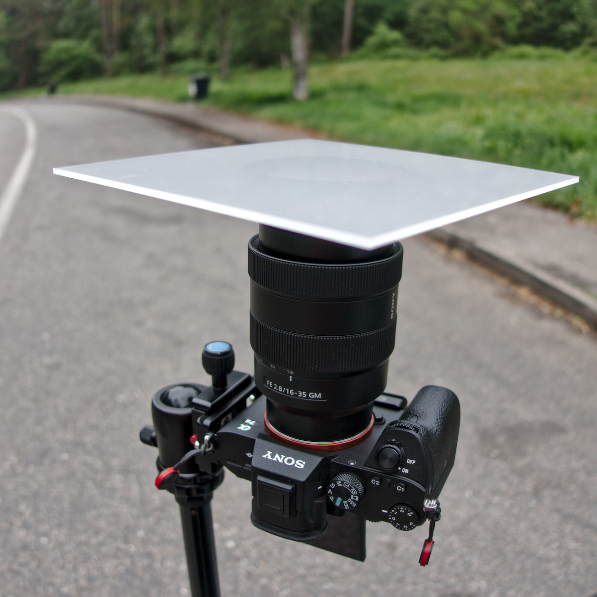
To create pictures for vignetting you need a diffuser in front of the lens. This
may be translucent milk glass, or white plastic foil on glass. Whatever, as
long as it is opaque enough so that nothing can be seen through it, yet
transparent enough so that light can pass through it. It must not be thicker
than 3 mm and shouldn’t have a noticeable texture. It must be perfectly flush
with the lens front, and it mustn’t be bent. It must be illuminated
homogeneously.
However white plastic foil taped on a piece of ordinary glass for stability
might be enough, if the plastic doesn’t have any texture.
I normally wait for a cloudy day with no sun, then the sky is homogeneously
lit. Put the camera on a tripod and point it to the sky. Put the glass directly
on the lens (remove any filters). In some places where sunlight is different
you may need to shoot indoors. You should experiment to make sure your images
are evenly lit (except for vignetting obviously).
Figure 6: Camera setup to take pictures for vignetting correction
Figure 6: Image showing vignetting of a wide angle lens at 16mm
Make sure that no corrections are applied by the camera (some models do
this even for RAWs). Set the camera to aperture priority and the
lowest real ISO (this is normally 100 or 200, don’t use extended ISO values).
Switch to manual focus and focus to infinity. This is the most critical step!
For zoom lenses, you need to take pictures at five different focal lengths. You
only need pictures for five focal lengths because for the other steps it gets
interpolated. For a prime lens you need to take only pictures for the single
focal length.
Take the pictures as RAW at the fastest aperture (e.g. f/2.8) and at three more
closed apertures at 1 EV distance, and also at the most closed aperture (e.g.
f/22.0). These are often marked on your lens’ aperture ring, or on your
electronic display.
If you have for example a 16-35mm lens with aperture f/2.8 - f/22, you need to
take pictures at 16mm, 20mm, 24mm, 28mm and 35mm focal length (Remember you
require the min and max zoom values). For each for those focal lengths you need
to take five pictures at f/2.8, f/4.0, f/5.6, f/8.0 and f/22.0. This makes 25
pictures in total.
For a 50mm prime lens with f/1.4 - f/16 you need to take 5 pictures at f1.4, f/2.0,
f/2.8, f/4.0, and f/16.0.
**Exposing the picture correctly
For taking the picture the middle of the area needs to be as bright as
possible, but not overexposed. This can be easily +1.7 to +2.0 EV.
If your camera has a zebra setting, turn it on and set the zebra mode to ‘100’.
If you start to see the zebra, then take the picure. The profile is created on
a RAW file and the zebra is shown for a developed picture. So we aren’t
overexposed yet. In the control mode in my camera which shows overexposure
everything was fine.
Vignetting correction for the professionals
The following steps are to get really fine grained vignetting corrections. The
gain in accuracy is really very small! I probably only makes sense for prime
lenses used for portrait or macro photography. However this is not required,
the above it absolutely enough.
Lensfun is able to correct vignetting depending on focal distance. Thus, you
can achieve a bit more accuracy by shooting at different focal distances. This
means you will have to take pictures at 4 different focal distances.
The first focus on the near point (The near point is the closest distance that
can be brought in focus). The next focal distances are the near point
multiplied by 2 and by 6 and finally focus at infinity.
Example: For a 85mm prime lens with the near point at 0.8 m. You have to take
pictures at 0.8 m, 1.6 m, 4.8 m and infinity.
Create calibration data
There are two ways to perform the calibration.
Lensfun allows an upload of data to the project, and they’ll do the program
work for you. They’ll also review your images to make sure they are correctly
taken.
Or you can do it yourself with the lens calibration script from the lensfun
project.
The script needs the following dependencies to be installed on your system:
You can download the lens calibration script
HERE or get it as a package
for the major distributions
HERE.
Once you have downloaded the tool create a folder for your lens calibration
data, change to the directory and run:
$ lens_calibrate.py init
The following directory structure has been created in the local directory

1. distortion - Put RAW file created for distortion in here
2. tca        - Put chromatic abbreviation RAW files in here
3. vignetting - Put RAW files to calculate vignetting in here
Follow the instructions and copy your raw files in the corresponding
directories.
Vignetting correction for the professionals
For each focal distance you captures pictures you have to create a folder.
Lets pick up the example from above. For a 85mm prime lens we took pictures at
0.8 m, 1.6 m, 4.8 m and infinity. For this lens you would have to create the
following folder structure in the vignetting directory:
The folder inf is for the focal distance at infinity.
Distortion
Once you copied the files in place it is time to generate the pictures (tif
files) for distortion calculations. You can do this with the
‘distortion’ option:
$ lens_calibrate.py distortion
Running distortion corrections ...
Converting distortion/_7M32376.ARW to distortion/exported/_7M32376.tif ... DONE
A template has been created for distortion corrections as lenses.conf.
Once the tif files has been created, you can start Hugin.
Torsten Bronger created a screen cast to give an overview about the distortion
process in Hugin. He uses an old Hugin version in the video. The following
section of this tutorial explains how to do it with Hugin 2018. You can watch
the screen cast first if you want, you can do it
here (Vimeo).
If you start Hugin the first time, the windows you will get should look like in
Figure 8.
Figure 8: Hugin start screen
First select on the menu bar Interface -> Expert to switch to the Expert
mode. You will get a windows which should look like as in Figure 9.
Figure 9: Hugin expert mode
Once in the export mode click on Add images (Figure 10) and load the first
tiff from the distortion/exported folder.
Figure 10: Adding images and setting the focal length and crop factor
By default the lens type should be set to Normal (rectiliniar) for normal
standard lenses. Make sure that the focal length is correct and set the Focal
length multiplier, which is the crop factor of your camera. For full frame
bodies this value should be 1. If you have a crop camera you need to set the
correct crop value you can find in the specifications. Next click on the
Control Points tab (Figure 11).
Figure 11: The control points tab
This is the tab to set the control points so that we can tell the software what
are our straight lines we are interested in. In this tab you have to make sure
that auto fine-tune is disabled, auto add is enabled and auto-estimate is
disabled! If this is the case zoom the image to 200% (you can also do this by
pressing ‘2’ on the keyboard).
In the zoomed images you have start at the top edges. On the left go to the top
left corner and to the top right corner on the right. The first straight line,
from left to right, should be visible. Select the first control point on
the left edge of the picture on the left page and the right edge on the
right (Figure 12).
Figure 12: Setting the first two control points for the line to add
IMPORTANT: Once you have the first control point selected in both images.
Select Add new Line in the mode dropdown menu! This will add the two
control points as line 3! Now continue adding corresponding control points in
both pictures till you’re in the middle on both sides.
Tip: The easiest and fasted is to set control points in the middle at the
tiling line. This reduces the required mouse movements.
Now zoom out by pressing ‘0’ and check it if everything has been added
correctly (Figure 13).
Figure 13: Control points for line3
While you are zoomed out, find a line which is about 3rd into the image from
the top to repeat adding a line. Zoom to 200% again, select the first control
points and again Add a new line which will result in line4 (Figure 14)!
Figure 14: Control points for line 3 and line 4
Zoom out by pressing ‘0’ and check that you have two lines, line3 and line4. Now move on to the Stitcher tab (Figure 14).
Figure 15: The stitcher tab, select the correct projection here.
In the Stitcher tab you need to select the correct Projection for your
lens. This is Rectilinear for standard lenses. Once done switch to the
Photos tab (Figure 16).
Figure 16: Enable the Optimizer tab.
At the bottom under Optimize select Custom parameters for Geometric.
This will add an Optimizer tab. Switch to it once it appears (Figure 17).
Figure 17: Optimizer tab: Select a b c for barrel distortion correction
Select the ‘a’, ‘b’ and ‘c’ lens parameters and click on Optimize now!.
Accept the calculation with yes. Now the values for ‘a’, ‘b’ and ‘c’ will
change (Figure 18).
Figure 18: Calculated distortion correction ‘a’, ‘b’ and ‘c’.
The calculated correction values for ‘a’, ‘b’ and ‘c’ you can find in the tab
need to be added to the lenses.conf. Open The file and fill out the missing
options. Here is an example:
Example:
[FE 85mm F1.4 GM]
maker = Sony
mount = Sony E
cropfactor = 1.0
aspect_ratio = 3:2
type = normal
maker is should be the lens manufacturer e.g. Sony
mount is the mount system for the lens, check the lensfun database
cropfactor is 1.0 for full frame cameras, if you have a crop camera find out the correct crop factor for it.
aspect_ratio is the aspect ratio for the pictures which is normally 3:2.
type is the type of the lens, e.g. ‘normal’ for standard rectilinear lenses. Other values are: stereographic, equisolid, stereographic, panoramic or fisheye.
If you have e.g. a 85mm there should be an entry for the focal length which is
set to: 0.0, 0.0, 0.0. You need to change the values in the lenses.conf for
your focal length with the calculated corrections from the Optimizer tab
(Figure 16).
[FE 85mm F1.4 GM]
maker = Sony
mount = Sony E
cropfactor = 1.0
aspect_ratio = 3:2
type = normal
distortion(85mm) = 0.002, 0.001, -0.009
But I don’t want to do distortion corrections!
No problem, if you want to skip this step then you can created the lenses.conf
manually. It should look like the following example:
[lens model]
maker =
mount =
cropfactor = 1.0
aspect_ratio = 3:2
type = normal
The section name is the lens model. You can find it out by running:
exiv2 -g LensModel -pt <raw image file>
The other options are:
maker is should be the lens manufacturer e.g. Sony
mount is the mount system for the lens, check the lensfun database
cropfactor is 1.0 for full frame cameras, if you have a crop camera find out the correct crop factor for it.
aspect_ratio is the aspect ratio for the pictures which is normally 3:2.
type is the type of the lens, e.g. ‘normal’ for standard rectilinear lenses. Other values are: stereographic, equisolid, stereographic, panoramic or fisheye.
TCA
You can skip this step if you don’t want to do TCA corrections.
This step is fully automatic, all you have to do is to run the following
command and wait:
$ lens_calibrate tca
Running TCA corrections for tca/exported/_7M32375.ppm ... DONE
However it possible to calculate more complex TCA corrections. For this you
need to run the step it with an additional command line argument, like this:
You can skip this step if you don’t want to do vignetting corrections.
To calculate the vignetting corrections it is also a very simple step. All you
have to do is to run the following command and wait:
$ lens_calibrate vignetting
Generating the XML
To get corrections for lensfun you need a lenses.conf with the required options
to be filled out (maker, mount, cropfactor, aspect_ratio, type). And at least
one of the corrections steps done. If you have this you can generate the XML
file which can be consumed by lensfun. You can do it with the following
command:
You can redo this step as many times as you want. And you can just rerun it if
you add an additional correction.
Using the lensfun.xml
You may want to fine-tune the lens model name in the generated lensfun.xml
file. Lensfun normalises names before any matching, so you have some freedom.
For example, upper/lowercase can be changed arbitrarily. Any single f is
ignored, so you may change 16-35mm 2.8 into 16-35mm f/2.8. If there was a
tele converter involved, you must add “converter” into the name so that Lensfun
does not try to derive allowed focal lengths from the lens name.
Ordering of parts in the lens name is completely unimportant for matching. As
are single punctuation characters. You may even add things (e.g. 16-35 into
16-35mm) but be conservative here. Never drop anything what exiv2 reports!
If you want to use the generated lensfun.xml file to test if the calibration
you created works, you can copy to the local lensfun config folder in your home
directory.
cp lensfun.xml ~/.local/share/lensfun
Make sure your camera is recognized by lensfun or you need to add an entry to
the lensfun.xml file too.
Contributing your lensfun.xml
To contribute your calibration data data for your lens to the lensfun project,
execute the script with the following command:
$ lens_calibrate ship
Created lensfun_calibration.tar.xz
Open a bug at https://github.com/lensfun/lensfun/issues/ with the data.
This will create a tarball with all the required data. Now go to
Please add the attached lens data to the lensfun data base.
Attach the lensfun_calibration.tar.xz to the bugreport.
Feedback
Feedback for this article is very welcome. If you’re a lensfun developer and
read this please contact me. I would like to contribute the script to lensfun
and further improve the article. I still have unanswered questions.
Mary Beard joins us to answer the question: Is it accurate to call Donald Trump a fascist?, while the TLS's fiction and politics editor Toby Lichtig discusses how the President is presented, in books and on film; and Julia Bell looks back on her Oxford entrance interview - with no fondness - and wonders: "Was it a trap or a test?"
Books
Fear: Trump in the White House by Bob Woodward
The Fifth Risk by Michael Lewis
Nobody hates Trump more than Trump by David Shields
To mark the centenary of the end of the First World War, the TLS's History editor David Horspool talks us through books, exhibitions and events that commemorate cataclysmic slaughter and scars that endure to this day; it’s easy to think of privacy invasion as a peculiarly modern phenomenon, but it has its own history dating back to the American Civil War – Sarah Igo tells us more; finally, the food writer Bee Wilson discusses two new cookbooks that capture a “fresh mood of experiment in the kitchen”
Works discussed
Pandora’s Box: A history of the First World War, by Jörn Leonhard (translated by Patrick Camiller)
Robert Graves: From Great War poet to ‘Good-Bye to All That’, 1895–1929 by Jean Moorcroft Wilson
Making a New World (across the Imperial War Museum, London, and the Imperial War Museum North)
Plus reviews and original pieces published in the TLS, including “What did Tommy read: The complex mental worlds of soldiers on the Western Front” by Bill Bell – go to the-TLS.co.uk for details
Sight Smell Touch Taste Sound: A new way to cook by Sybil Kapoor
As Mike Leigh's film of the Peterloo massacre of 1819 is released, Clare Pettitt revisits the history; Marina Benjamin offers a personal and literary account of the threshold between sleep and wakefulness; following the publication of a second volume of Sylvia Plath's letters, Hannah Sullivan looks for fresh insights into the poet's work, life and death; finally, Sam Riviere reads his new poem, "Sushi Tuesday"
Works discussed
Peterloo, directed by Mike Leigh
Insomnia by Marina Benjamin
The Letters of Sylvia Plath Volume I (1940-1956) and Volume II (1956-1963), edited by Peter K. Steinberg and Karen V. Kukil
Are authors, reviewers and publicists wasting their time on book coverage? The contemporary conversation about books and ideas goes way beyond traditional features and interviews. Book groups, academic seminars, Amazon user reviews, Goodreads, the press, radio, podcasts, and sometimes even TV: the form, tone and quality of coverage has infinite variety. But how much does any of it help the books business – if it can be measured at all? Do authors, reviewers, and publicists feel their efforts are worthwhile? Michael Caines, an editor at the TLS, chairs an eclectic panel for a crucial conversation about the conversation around books. (This a live recording of an event, in collaboration with BookMachine, which took place on October 3, 2018, at the Driver, Kings Cross, London)
Elaine Showalter on a history of obscenity and censorship and the largely futile efforts of a US Postal Inspector; Ladee Hubbard on five years of Black Lives Matter and the myth of an egalitarian, post-racial America; Kassia St Clair on women, weaving and the rewriting of history
Books
Lust on Trial: Censorship and the rise of obscenity in the age of Anthony Comstock by Amy Werbel
The Fire This Time: A new generation speaks about race, edited by Jesmyn Ward
My Brother Moochie: Regaining dignity in the face of crime, poverty and racism in the American South by Isaac J. Bailey
The Golden Thread: How fabric changed history by Kassia St Clair
Keith Miller joins us to discuss everybody's favourite Renaissance man; the TLS's Fiction editor Toby Lichtig meets Anna Burns, the winner of the 2018 Man Booker Prize for her novel Milkman; this year's Nobel Prize for Literature, meanwhile, remains suspended following charges of serious sexual misconduct and cronyism – Richard Orange reports on the mess that has engulfed the Swedish Academy
Books
Living with Leonardo: Fifty years of sanity and insanity in the art world and beyond by Martin Kemp
Mary Beard reflects on the peculiarities of Homer's best-loved, many-sided epic; Neel Mukherjee on the scandalous survival of the Indian caste system; following the recent party conferences, James O'Brien offers a wry overview of Britain's political mess
Books:
The Measure of Homer: The ancient reception of the Iliad and the Odyssey by Richard Hunter
Ants Among Elephants: An untouchable family and the making of modern India by Sujatha Gidla
How To Be Right ... in a World Gone Wrong by James O'Brien
Michael Caines joins us to discuss female liberation in genteel Cheltenham; we look ahead to an Odyssey extravaganza, with Ted Hodgkinson from the Southbank centre; Paul Muldoon brings a salutary note of optimism to US politics and history with his new poem "With Joseph Brant in Canajoharie"
Books
Votes for Women: Cheltenham and the Cotswolds by Sue Jones
In this bonus episode, the TLS's History editor David Horspool discusses Thomas Cromwell with Diarmaid MacCulloch, the author of a new, definitive biography.
Lorna Scott Fox joins us to discuss the fiftieth anniversary of Mexico's Tlatelolco of 1968, a travesty still shrouded in obfuscation; the TLS's History editor David Horspool discusses Thomas Cromwell with Diarmaid MacCulloch, the author of a new, definitive biography; and finally, Rozalind Dineen offers a round-up of interesting new podcasts
Books and podcasts discussed
México 68: The students, the President and the CIA by Sergio Aguayo
Andrea is developing Photo Flow, GIMP AppImage, Hugin AppImage, and more!
Andrea Ferrero, or as we know him Carmelo_DrRaw, has been contributing to the PIXLS.US community since April of 2015. A self described developer and photography enthusiast, Andrea is the developer of the PhotoFlow image editor, and is producing AppImages for:
The GIMP image manipulation program - weekly AppImage packages from stable releases and development branches.
The Hugin panorama photo stitcher - AppImages for stable releases and development branches
Andrea is the best sort of community member, contributing six different projects (including his own)! He is always thoughtful in his responses, does his own support for PhotoFlow, and is kind and giving. He has finally started a Patreon page to support his all of his hard work. Support him now!
He was also kind enough to answer a few questions for us:
PX: When did you get into photography? What’s your favorite subject matter?
AF: I think I was about 15 when I got my first reflex, and I was immediately fascinated by macro-photography. This is still what I like to do the most, together with taking pictures of my kids. ;-)
By the way, you can visit my personal free web gallery on GitHub: http://aferrero2707.github.io/photorama/gallery/ (adapted from this project).
It is still a work in progress, but you are welcome to fork it and adapt it to your needs if you find it useful!
PX: What brought you to using and developing Free/Open Source Software?
AF: I started to get interested in programming when I was at the university, in the late 90’s. At that time I quickly realized that the easiest way to write and compile my code was to throw Linux into my hard drive. Things were not as easy as today but I eventually managed to get it running, and the adventure began.
A bit later I started a scientific career (nothing related to image processing or photography, so I won’t bother with more details about my daily job), and since then I have been a user of Linux-based computing clusters for almost 20 years at the time of writing… A large majority of the software tools I use at work are free and open sourced and this definitely has marked my way of thinking and developing.
PX: What are some new/exciting features you develop in Photo Flow?
AF: Currently I am mostly focusing on HDR processing and high-quality Dynamic Range compression - what is also commonly called shadows/highlights compression.
More generally, there is still a lot of work to do on the performances side. The software is already usable and quite stable, but some of the image filters are still a bit too slow for real-time feedback, especially when combined together.
The image exporting module is also currently in a state of work in progress. It is already possible to select either Jpeg or TIFF (8, 16 or floating-point 32 bits bit depth) as the output format, to resize the image and add some post-resize sharpening, and to select the output ICC profile.
What is still missing is a real-time preview of the final result, with a possibility to soft-proof the output profile. The same options need to be included in the batch processor as well.
On a longer term, and if there is some interest from the community, I am thinking about porting the code to Android in a simplified form that would be suitable for tablets and the like. The small memory footprint of the program could be an important advantage on such systems.
PX: What other applications would you like to make an AppImage for? Have you explored Snaps or Flatpaks?
AF: I am currently developing and refining AppImage packages for GIMP, RawTherapee, LuminanceHDR and HDRMerge, in addition to PhotoFlow. All packages are automatically built and deployed through Travis CI, for better reproducibility and increased security. Hugin is the next application that I plan to package as an AppImage.
All the AppImage projects are freely available on GitHub. That’s also the best place for any feedback, bug report, or suggestion.
There is an ongoing discussion with the GIMP developers about the possibility to provide the AppImage as an official download.
In addition to the AppImage packages, I am also working with the RawTherapee developers on cross-compiled Windows packages that are also automatically built on Travis CI. The goal is to help them provide up-to-date packages from the main development branches, so that more users can test them and provide feedback.
I’m also open to any suggestions for additional programs that could be packaged as AppImages, so do not hesitate to express your wishes!
Personally I am a big fan of the AppImage idea, mostly because, unlike Snap or Flatpack packages, it is not bound to any specific distribution or run-time environment. The packager has full control over the contents of the AppImage package, pretty much like MacOS bundles.
Moreover, I find the community of developers around the AppImage format very active and open-minded. I am currently collaborating to improve the packaging of GTK applications. For those who are interested in the details, the discussion can be followed here: https://github.com/linuxdeploy/linuxdeploy/issues/2
Philip Horne and Frances Wilson join us to discuss Henry James, the not-always masterly Master who gave us novels as apparently divergent as Washington Square, with its clear, tight prose, The Ambassadors (prone to accidents of publication) and The Golden Bowl, which spills pleasures of an altogether more sinuous nature; plus, details of a little-known trip James took to California, which – unexpectedly, perhaps –“completely bowled” him over
Books
Generous Mistakes: Incidents of error in Henry James by Michael Anesko
The Cambridge Edition of the Complete Fiction of Henry James: The Ambassadors; Edited by Nicola Bradbury. The Portrait of a Lady; Edited by Michael Anesko. The Jolly Corner and Other Tales, 1903–1910; Edited by N. H. Reeve (Michael Anesko, Tamara L. Follini, Philip Horne and Adrian Poole, general editors)
Roz Dineen on the time-stained image of the artist-addict, The Recovering by Leslie Jamison, and whether “stories about getting better [can] ever be as compelling as stories about falling apart"; "David Foster Wallace would send me letters and I wouldn’t answer them. He would send works in progress with forlorn notes. 'You’re under no obligation to read or to pretend you’ve read the enclosed,' he wrote on one piece. I didn’t." – David Streitfeld recalls being David Foster Wallace's "worst friend"
Books
The Recovering by Leslie Jamison
In The Realm of Hungry Ghosts: Close encounters with addiction by Gabor Maté
Andrew Motion discusses the life, work and curious afterlife of his friend and "subject" Philip Larkin; Imogen Russell Williams has written an essay on diversity (or the lack of it) in children's books and offers some recommendations; Zoe Williams gives her verdict on the very British political tradition that is Prime Minister’s Questions
Books
Philip Larkin: A writer's life by Andrew Motion (1993; reissued September 2018)
The Poet X by Elizabeth Acevedo
Square by Mac Barnett and Jon Klassen
I Am Thunder by Muhammad Khan
Knights and Bikes by Gabrielle Kent
You’re Safe With Me by Chitra Soundar and Poonam Mistry
Knights and Bikes by Gabrielle Kent
You’re Safe With Me by Chitra Soundar and Poonam Mistry
(For all the books discussed by Imogen Russell Williams, go to the-tls.co.uk)
Punch and Judy Politics: An insider’s guide to Prime Minister’s questions by Tom Hamilton and Ayesha Hazarika
The IMAGE team of the GREYC laboratory is happy to celebrate the 10th anniversary of G’MIC with you, an open-source (CeCILL), generic and extensible framework for image processing.
GREYC is a public research laboratory on digital technology located in Caen, Normandy/France, under the supervision of 3 research institutions: the CNRS (UMR 6072), the University of Caen Normandy and the ENSICAEN engineering school.
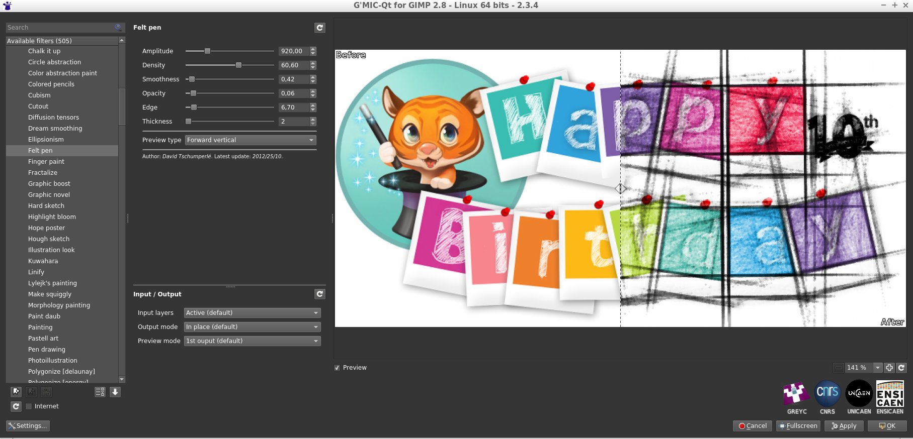
G’MIC-Qt, the main user interface of the G’MIC project.
This celebration gives us the perfect opportunity to announce the release of a new version (2.3.6) of this free software and to share with you a summary of the latest notable changes since our last G’MIC report, published on PIXLS.US in February 2018.
G’MIC is a multiplatform framework (GNU/Linux, macOS, Windows…) providing various user interfaces for manipulating generic image data, such as 2D or 3D hyperspectral images or image sequences with float values (thus including “normal” color images). More than 1000 different operators for image processing are included, a number that is extensible at will since users can add their own functions by using the embedded script language.
It was at the end of July 2008 that the first lines of G’MIC code were created (in C++).
At that time, I was the main developer involved in CImg, a lightweight open sourceC++ library for image processing, when I made the following observation:
The initial goal of CImg, which was to propose a “minimal” library of functions to help C++ developers to develop image processing algorithms, was broadly achieved; most of the algorithms I considered as essential in image processing were integrated. CImg was initially meant to stay lightweight, so I didn’t want to include new algorithms ad vitam æternam, which would be too heavy or too specific, thus betraying the initial concept of the library.
However, this would only cater to a rather small community of people with both C++ knowledge and image processing knowledge! One of the natural evolutions of the project, creating bindings of CImg to other programming languages, didn’t appeal much to me given the lack of interest I had in writing the code. And these potential bindings still only concerned an audience with some development expertise.
My ideas were starting to take shape: I needed to find a way to provide CImg processing features for non-programmers. Why not attempt to build a tool that could be used on the command line (like the famous convert command from Imagemagick)? A first attempt in June 2008 (inrcast, presented on the French news site LinuxFR), while unsuccessful, allowed me to better understand what would be required for this type of tool to easily process images from the command line.
In particular, it occurred to me that conciseness and coherence of the command syntax were the two most important things to build upon. These were the aspects that required the most effort in research and development (the actual image processing features were already implemented in CImg). In the end, the focus on conciseness and coherence took me much further than originally planned as G’MIC got an interpreter) of its own scripting language, and then a JIT compiler for the evaluation of mathematical expressions and image processing algorithms working at the pixel level.
With these ideas, by the end of July 2008, I was happy to announce the first draft of G’MIC. The project was officially up and running!
Fig. 1.1: Logo of the G’MIC project, libre framework for image processing, and its cute mascot “Gmicky” (illustrated by David Revoy).
A few months later, in January 2009, enriched by my previous development experience on GREYCstoration (a free tool for nonlinear image denoising and interpolation, from which a plug-in was made for GIMP), and in the hopes of reaching an even larger public, I published a G’MICGTK plug-in for GIMP.
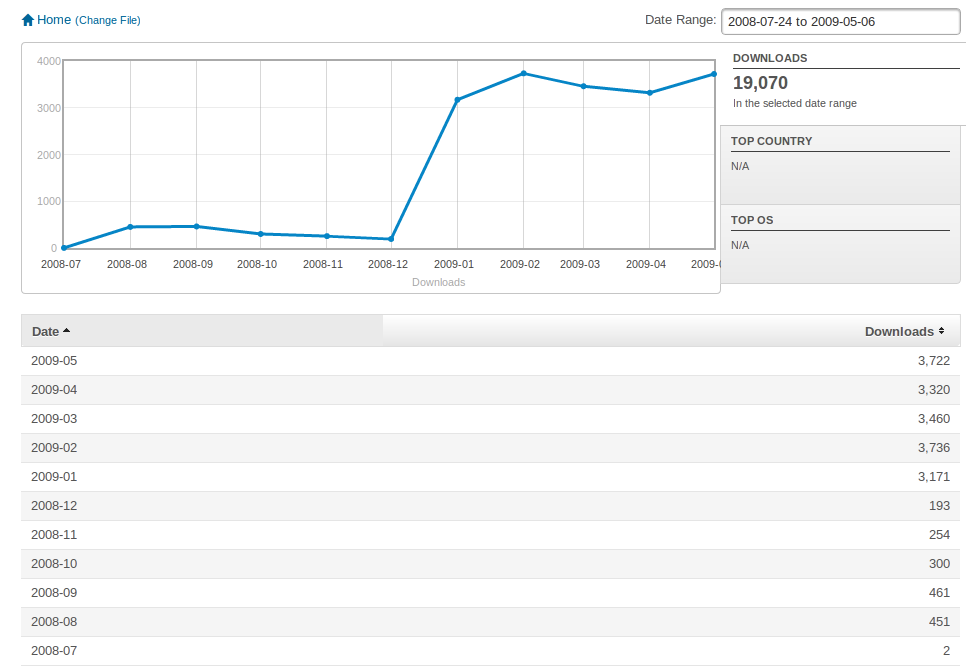
This step proved to be a defining moment for the G’MIC project, giving it a significant boost in popularity as seen below (the project was hosted on Sourceforge at the time).
Fig.1.2: Monthly downloads statistics of G’MIC, between July 2008 and May 2009 (release of the GIMP plug-in happened in January 2009).
The sudden interest in the plugin from different users of GIMP (photographers, illustrators and other types of artists) was indeed a real launchpad for the project, with the rapid appearance of various contributions and external suggestions (for the code, management of the forums, web pages, writing of tutorials and realization of videos, etc.). The often idealized community effect of free software finally began to take off! Users and developers began to take a closer look at the operation of the original command-line interface and its associated scripting language (which admittedly did not interest many people until that moment!). From there, many of them took the plunge and began to implement new image processing filters in the G’MIC language, continuously integrated them into the GIMP plugin. Today, these contributions represent almost half of the filters available in the plugin.
Meanwhile, the important and repeated contributions of Sébastien Fourey, colleague of the GREYC IMAGE team (and experienced C++ developer) significantly improved the user experience of G’MIC. Sébastien is indeed at the heart of the main graphical interface development of the project, namely:
The G’MIC Online web service (which was later re-organised by GREYC’s Development Department).
Free Software ZArt, a graphical interface - based on the _Qt_ library - for the application of G’MIC filters to video sequences (from files or digital camera streams).
And above all, at the end of 2016, Sébastien tackled a complete rewrite of the G’MIC plugin for GIMP in a more generic form called G’MIC-Qt. This component, also based on the _Qt_ library (as the name suggests), is a single plugin that works equally well with both GIMP and Krita, two of the leading free applications for photo retouching/editing and digital painting. G’MIC-Qt has now completely supplanted the original GTK plugin thanks to its many features: built-in filter search engine, better preview, superior interactivity, etc. Today it is the most successful interface of the G’MIC project and we hope to be able to offer it in the future for other host applications (contact us if you are interested in this subject!).
Fig.1.3: Different graphical interfaces of the G’MIC project, developed by Sébastien Fourey: G’MIC-Qt, G’MIC Online and ZArt.
The purpose of this article is not to go into too much detail about the history of the project. Suffice it to say that we have not really had time to become bored in the last ten years!
Today, Sébastien and I are the two primary maintainers of the G’MIC project (Sébastien mainly for the interface aspects, myself for the development and improvement of filters and the core development), in addition to our main professional activity (research and teaching/supervision).
Let’s face it, managing a free project like G’MIC takes a considerable amount of time, despite its modest size (~120k lines of code). But the original goal has been achieved: thousands of non-programming users have the opportunity to freely and easily use our image processing algorithms in many different areas: image editing, photo manipulation, illustration and digital painting, video processing, scientific illustration, procedural generation, glitch art…
The milestone of 3.5 million total downloads was exceeded last year, with a current average of about 400 daily downloads from the official website (figures have been steadily declining in recent years as G’MIC is becoming more commonly downloaded and installed via alternative external sources).
It is sometimes difficult to keep a steady pace of development and the motivation that has to go with it, but we persisted, thinking back to the happy users who from time to time share their enthusiasm for the project!
Obviously we can’t name all the individual contributors to G’MIC whom we would like to thank, and with whom we’ve enjoyed exchanging during these ten years, but our heart is with them! Let’s also thank the GREYC laboratory and INS2I institute of CNRS for their strong support for this free project. A big thank you also to all the community of PIXLS.US who did a great job supporting the project (hosting the forum and publishing our articles on G’MIC).
But let’s stop reminiscing and get down to business: new features since our last article about the release of version 2.2!
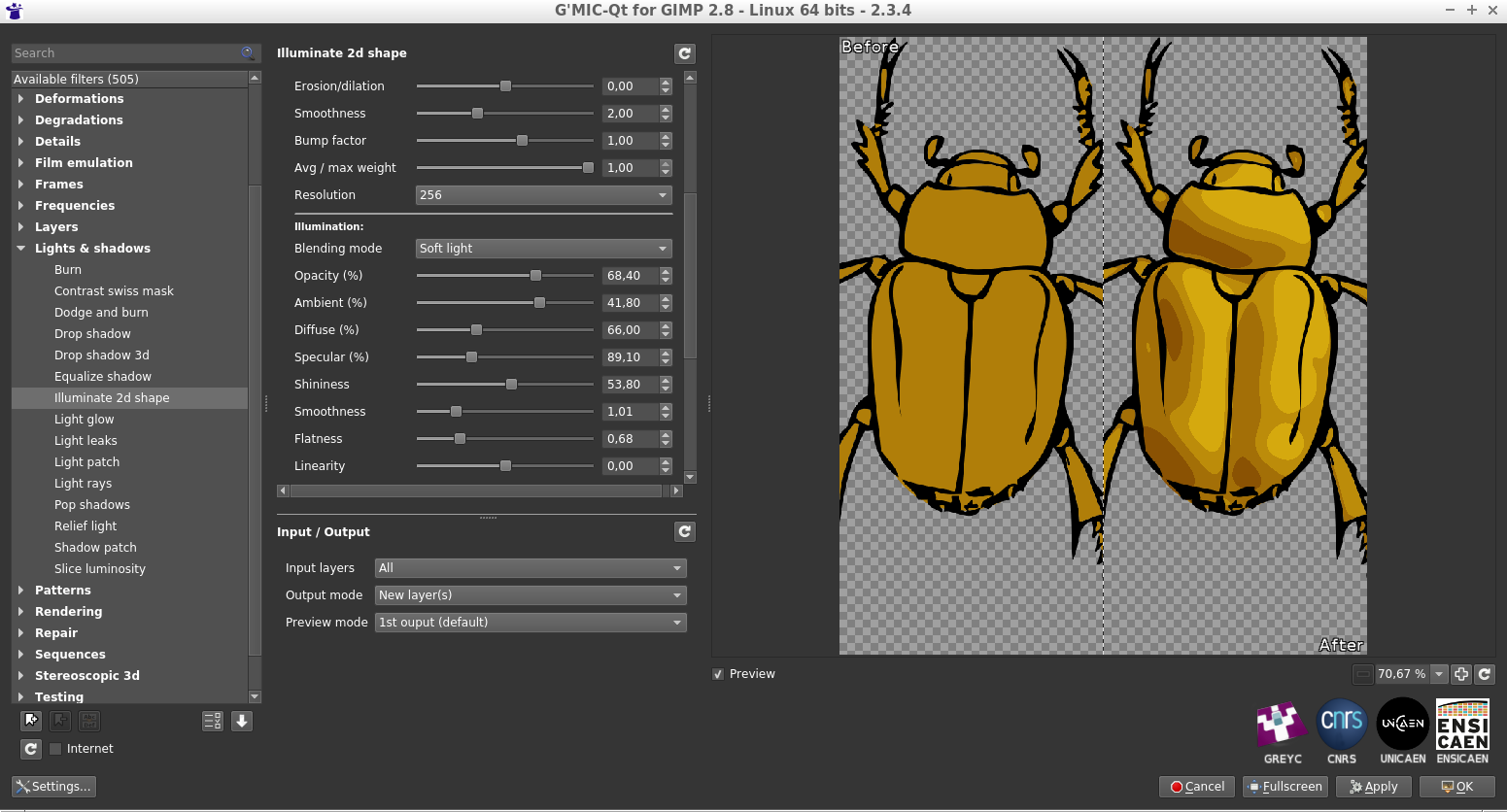
G’MIC recently gained a quite impressive new filter named « Illuminate 2D shape », the objective of which is to automatically add lit zones and clean shadows to flat-colored 2D drawings, in order to give a 3D appearance.
First, the user provides an object to illuminate, in the form of an image on a transparent background (typically a drawing of a character or animal). By analyzing the shape and content of the image, G’MIC then tries to deduce a concordant 3D elevation map (“ bumpmap “). The map of elevations obtained is obviously not exact, since a 2D drawing colored in solid areas does not contain explicit information about an associated 3D structure! From the estimated 3D elevations it is easy to deduce a map of normals (“ normalmap “) which is used in turn to generate an illumination layer associated with the drawing (following a Phong Shading model).
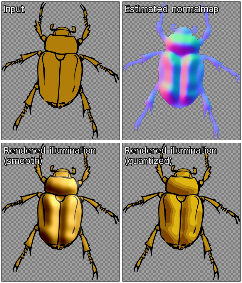
Fig. 2.1: G’MIC’s “Illuminate 2D shape“ filter in action, demonstrating automatic shading of a beetle drawing (shaded result on the right).
This new filter is very flexible and allows the user to have a fairly fine control over the lighting parameters (position and light source rendering type) and estimation of the 3D elevation. In addition the filter gives the artist the opportunity to rework the generated illumination layer, or even directly modify the elevation maps and estimated 3D normals. The figure below illustrates the process as a whole; using the solid colored beetle image (top left), the filter fully automatically estimates an associated 3D normal map (top right). This allows it to generate renditions based on the drawing (bottom row) with two different rendering styles: smooth and quantized.
Fig. 2.2: The process pipeline of the G’MIC “Illuminate 2D shape“ filter involves the estimation of a 3D normal map to generate the automatic illumination of a drawing.
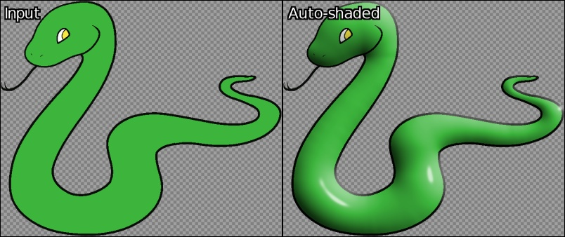
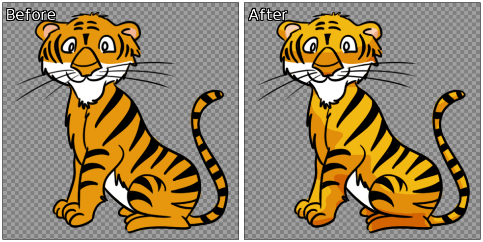
Despite the difficulty inherent in the problem of converting a 2D image into 3D elevation information, the algorithm used is surprisingly effective in a good many cases. The estimation of the 3D elevation map obtained is sufficiently consistent to automatically generate plausible 2D drawing illuminations, as illustrated by the two examples below - obtained in just a few clicks!
Fig. 2.3: Two examples of completely automatic shading of 2D drawings, generated by G’MIC
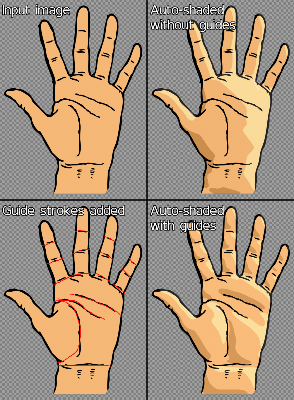
It occurs, of course, that the estimated 3D elevation map does not always match what one might want. Fear not, the filter allows the user to provide “guides” in the form of an additional layer composed of colored lines, giving more precise information to the algorithm about the structure of the drawing to be analyzed. The figure below illustrates the usefulness of these guides for illuminating a drawing of a hand (top left); the automatic illumination (top right) does not account for information in the lines of the hand. Including these few lines in an additional layer of “guides” (in red, bottom left) helps the algorithm to illuminate the drawing more satisfactorily.
Fig. 2.4: Using a layer of “guides” to improve the automatic illumination rendering generated by G’MIC.
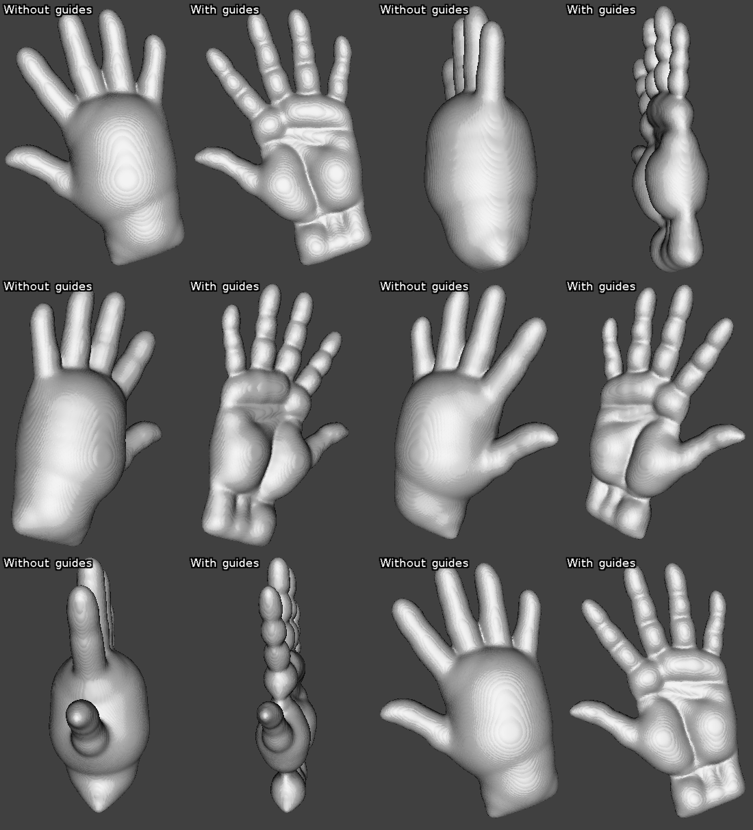
If we analyze more precisely the differences obtained between estimated 3D elevation maps with and without guides (illustrated below as symmetrical 3D objects), there is no comparison: we go from a very round boxing glove to a much more detailed 3D hand estimation!
Fig. 2.5: Estimated 3D elevations for the preceding drawing of a hand, with and without the use of “guides”.
Finally, note that this filter also has an interactive preview mode, allowing the user to move the light source (with the mouse) and have a preview of the drawing illuminated in real time. By modifying the position parameters of the light source, it is thus possible to obtain the type of animations below in a very short time, which gives a fairly accurate idea of the 3D structure estimated by the algorithm from the original drawing.
Fig. 2.6: Modification of the position of the light source and associated illumination renderings, calculated automatically by G’MIC.
A video showing the various possible ways to edit the illumination allowed by this filter is visible here. The hope is this new feature of G’MIC allows artists to accelerate the illumation and shading stage of their future drawings!
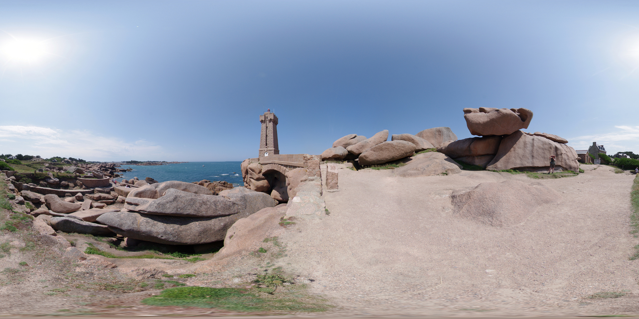
In a completely different genre, we have also added a filter implementing stereographic projection, suitably named “Stereographic projection“. This type of cartographic projection makes it possible to project planar defined image data onto a sphere. It should be noted that this is the usual projection used to generate images of “mini-planets” from equirectangular panoramas, like the one illustrated in the figure below.
Fig. 3.1: Example of equirectangular panorama (created by Alexandre Duret-Lutz).
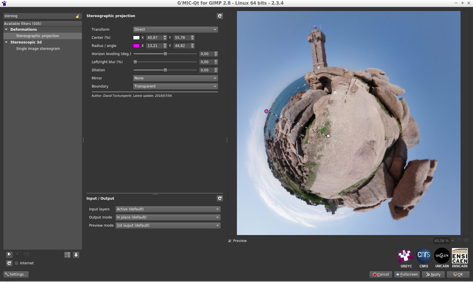
If we launch the G’MIC plugin with this panorama and select the filter “Stereographic projection“, we get:
Fig. 3.2: The “Stereographic projection“ filter of G’MIC in action using the plugin for GIMP or Krita.
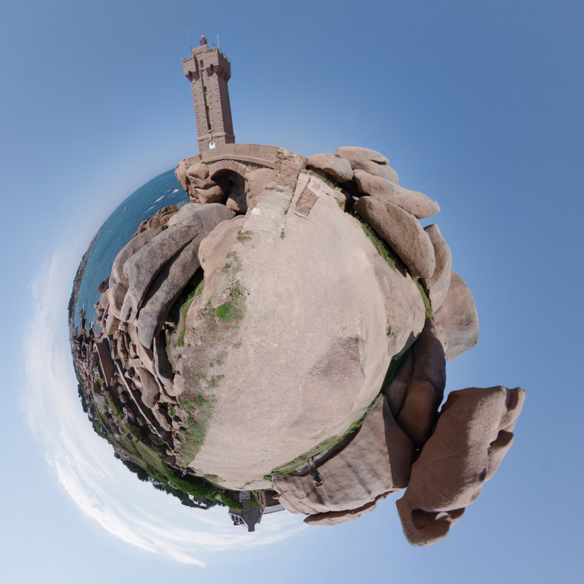
The filter allows precise adjustments of the projection center, the rotation angle, and the radius of the sphere, all interactively displayed directly on the preview window (we will come back to this later). In a few clicks, and after applying the filter, we get the desired “mini-planet”:
Fig. 3.3: “Mini-planet” obtained after stereographic projection.
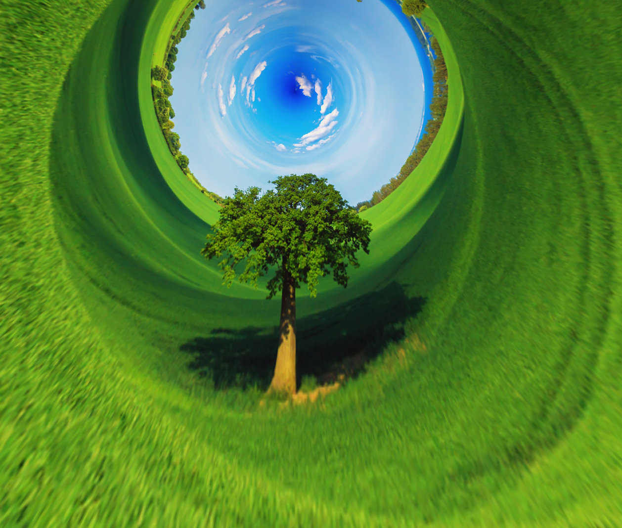
It is also intruiging to note that simply by reversing the vertical axis of the images, we transform a “mini-planet” into a “max-tunnel”!
Fig. 3.4: “Maxi-tunnel” obtained by inversion of the vertical axis then stereographic projection.
Again, we made this short video which shows this filter used in practice. Note that G’MIC already had a similar filter (called “Sphere“), which could be used for the creation of “mini-planets”, but with a type of projection less suitable than the stereographic projection now available.
Manipulating the colors of images is a recurring occupation among photographers and illustrators, and G’MIC already had several dozen filters for this particular activity - grouped in a dedicated category (the originally named “Colors“ category!). This category is still growing, with two new filters having recently appeared:
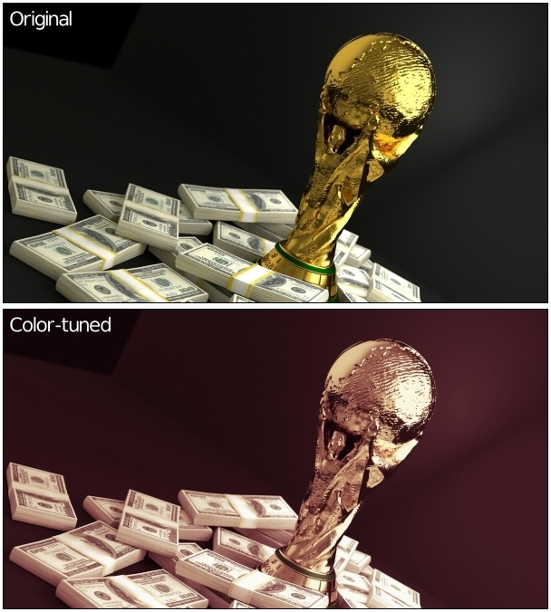
The “CLUT from after-before layers“ filter tries to model the color transformation performed between two images. For example, suppose we have the following pair of images:
Fig. 4.1: Pair of images where an unknown colorimetric transformation has been applied to the top image to obtain the bottom one.
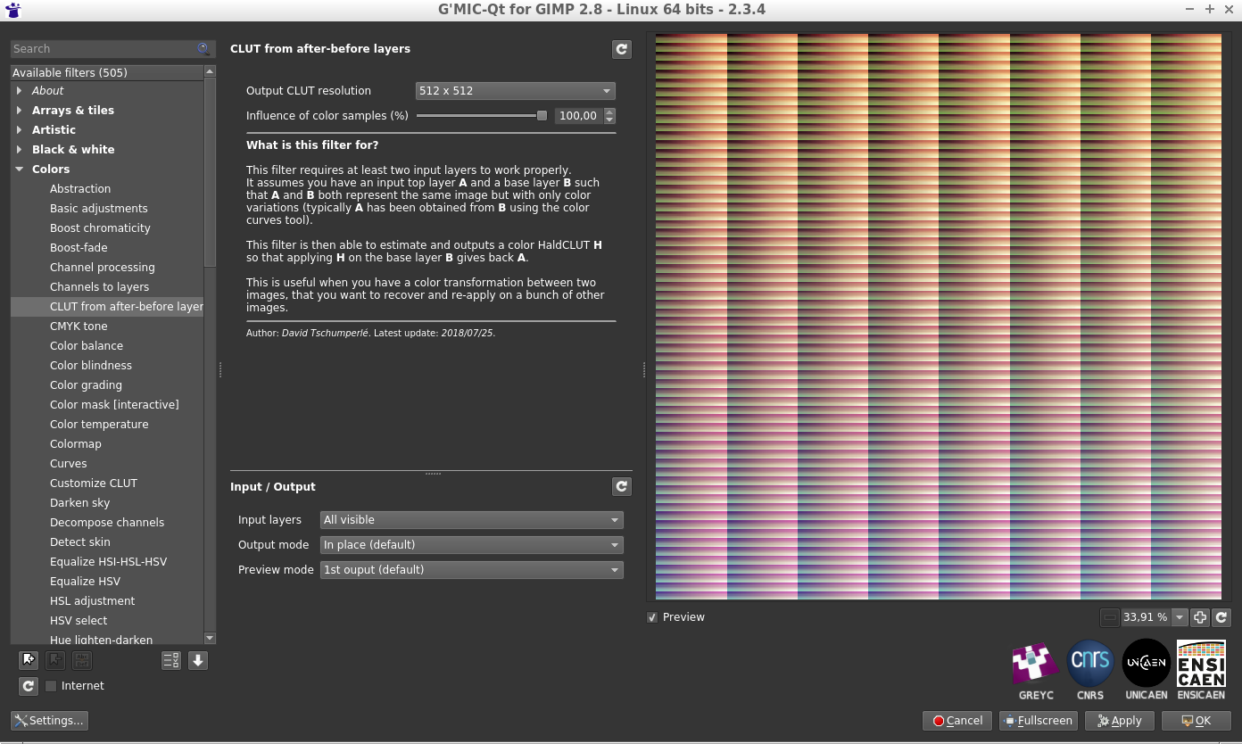
Problem: we do not remember at all how we went from the the original image to the modified image, but we would like to apply the same process to another image. Well, no more worries, call G’MIC to the rescue! The filter in question will seek to better model the modification of the colors in the form of a HaldCLUT, which happens to be a classic way to represent any colorimetric transformation.
Fig. 4.2: The filter models the color transformation between two images as a HaldCLUT.
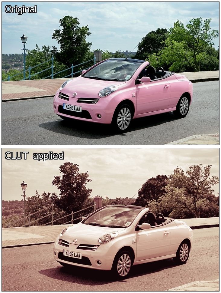
The HaldCLUT generated by the filter can be saved and re-applied on other images, with the desired property that the application of the HaldCLUT on the original image produces the target model image originally used to learn the transformation.
From there, we are able to apply an equivalent color change to any other image:
Fig. 4.3: The estimated color transformation in the form of HaldCLUT is re-applied to another image.
This filter makes it possible in the end to create HaldCLUT “by example”, and could therefore interest many photographers (in particular those who distribute compilations of HaldCLUT files, freely or otherwise!).
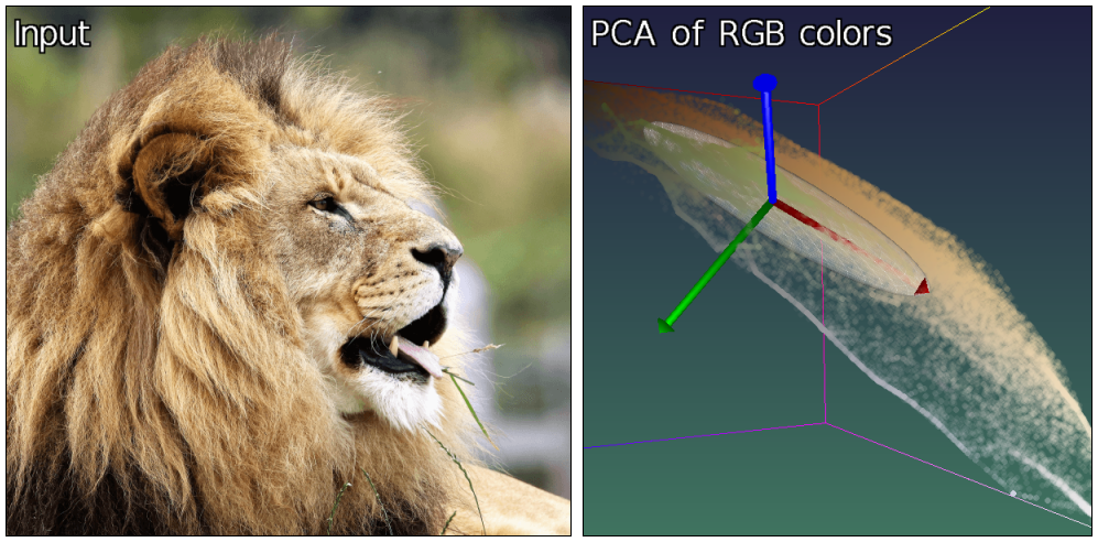
A second color manipulation filter, named “Mixer [PCA]“ was also recently integrated into G’MIC. It acts as a classic color channel mixer, but rather than working in a predefined color space (like sRGB, HSV, Lab…), it acts on the “natural” color space of the input image, obtained by principal component analysis (PCA) of its RGB colors. Thus each image will be associated with a different color space. For example, if we take the “lion” image below and look at the distribution of its colors in the RGB cube (right image), we see that the main axis of color variation is defined by a straight line from dark orange to light beige (axis symbolized by the red arrow in the figure).
Fig. 4.4: Distribution of colors from the “lion” image in the RGB cube, and associated main axes (colorized in red, green and blue).
The secondary axis of variation (green arrow) goes from blue to orange, and the tertiary axis (blue arrow) from green to pink. It is these axes of variation (rather than the RGB axes) that will define the color basis used in this channel mix filter.
Fig. 4.5: The “Mixer [PCA]“ filter is a channel mixer acting on the axes of “natural” color variations of the image.
It would be wrong to suggest that it is always better to consider the color basis obtained by PCA for the mixing of channels, and this new filter is obviously not intended to be the “ultimate” mixer that would replace all others. It simply exists as an alternative to the usual tools for mixing color channels, an alternative whose results proved to be quite interesting in tests of several images used during the development of this filter. It does no harm to try in any case…
This section is about a few other filters improved or included lately in G’MIC which deserve to be talked about, without dwelling too much on them.
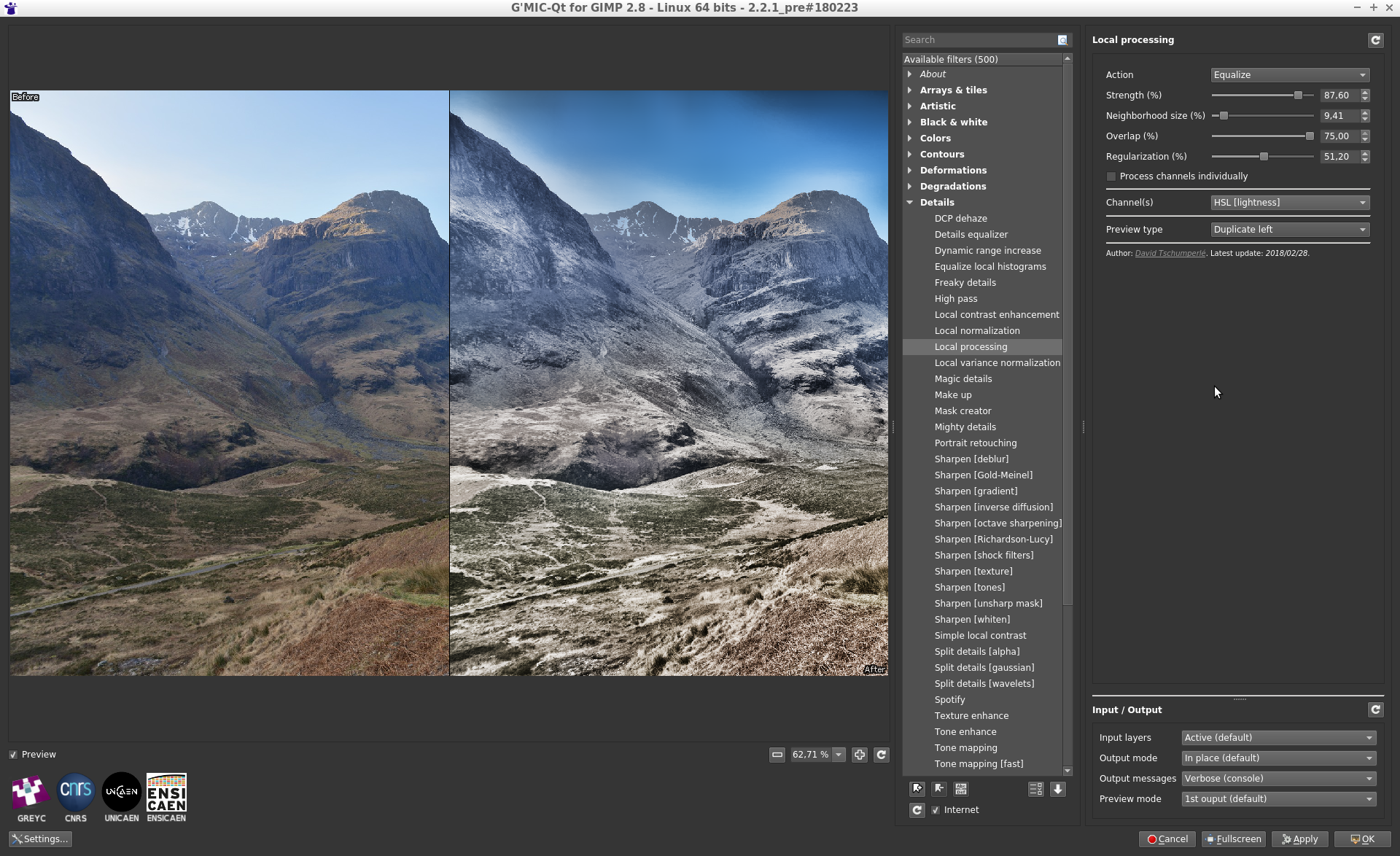
Filter “Local processing” applies a color normalization or equalization process on the local image neighborhoods (with possible overlapping). This is an additional filter to make details pop up from under or over-exposed photographs, but it may create strong and unpleasant halo artefacts with non-optimal parameters.
Fig. 5.1: The new filter “Local processing” enhances details and contrast in under or over-exposed photographs.
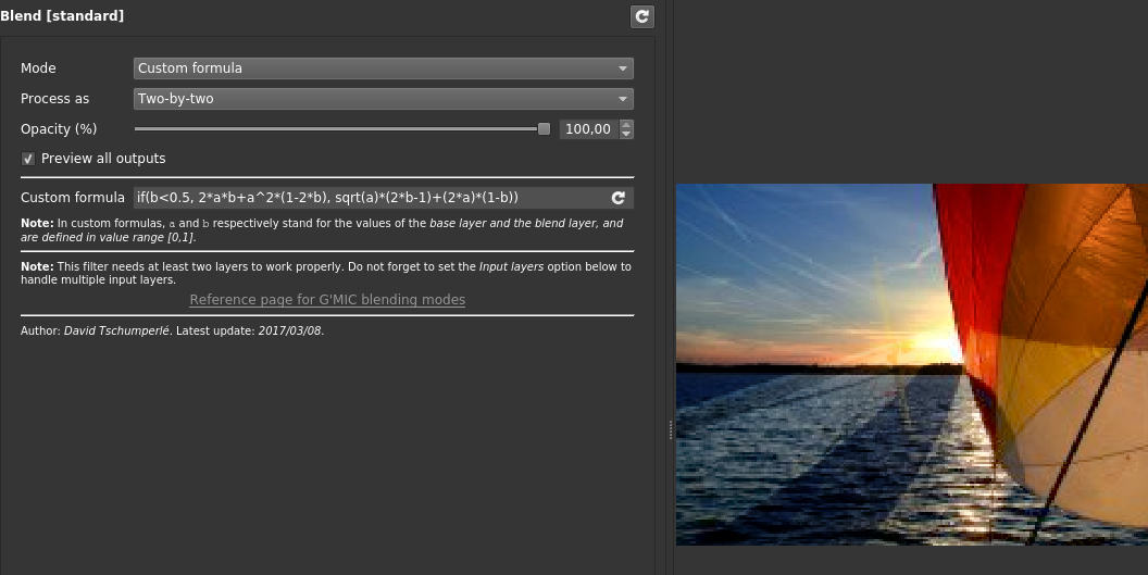
If you think that the number of layer blending modes available in GIMP or Krita is not enough, and dream about defining your own blending mode formula, then the recent improvement of the G’MIC filter « Blend [standard] » will please you! This filter now gets a new option « Custom formula » allowing the user to specify their own mathematical formula when blending two layers together. All of your blending wishes become possible!
Fig. 5.2: The “Blend [standard]“ filter now allows definition of mathematical formulas for layer merging.
Also note the complete re-implementation of the nice “Sketch“ filter, which had existed for several years but could be a little slow on large images. The new implementation is much faster, taking advantage of multi-core processing when possible.
Fig. 5.3: The “Sketch“ filter has been re-implemented and now exploits all available compute cores.
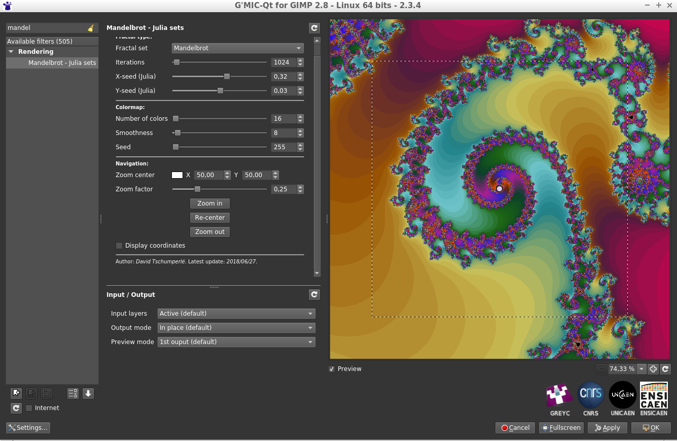
A large amount of work has also gone into the re-implementation of the “Mandelbrot - Julia sets“ filter, since the navigation interface has been entirely redesigned, making exploration of the Mandelbrot set much more comfortable (as illustrated by this video). New options for choosing colors have also appeared.
Fig. 5.4: The “Mandelbrot - Julia sets“ filter and its new navigation interface in the complex space.
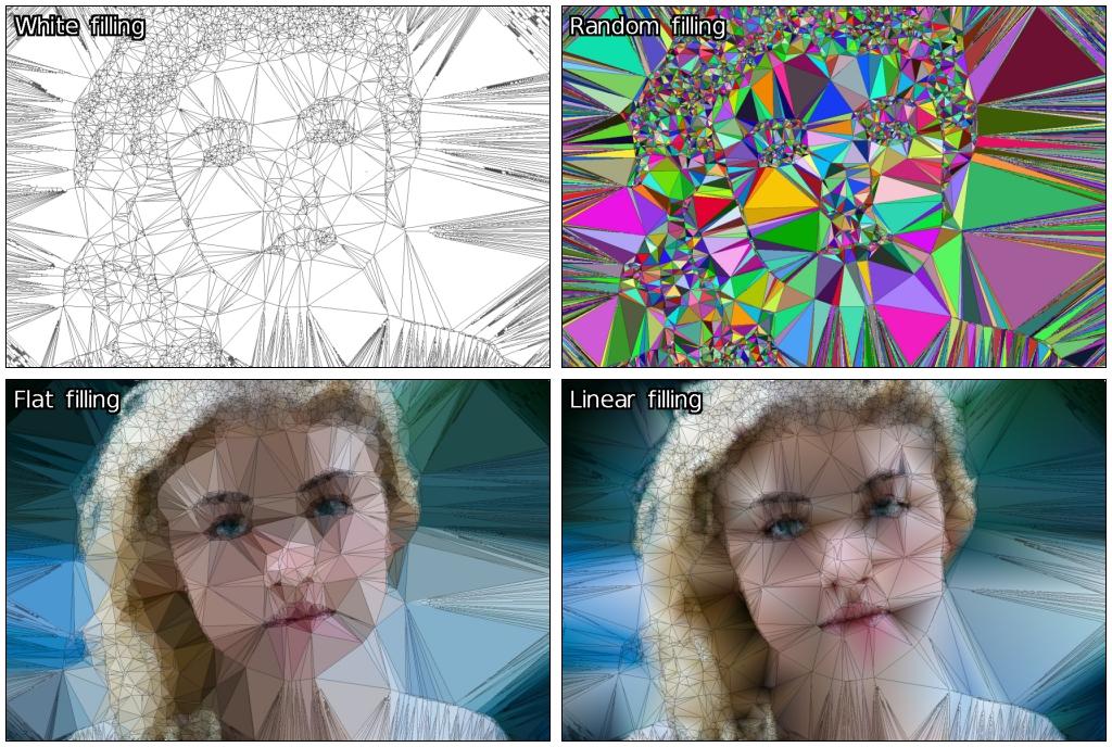
In addition, the “Polygonize [Delaunay]“ filter that generates polygonized renderings of color images has a new rendering mode, using linearly interpolated colors in the Delaunay triangles produced.
Fig. 5.5: The different rendering modes of the “Polygonize [Delaunay]“ filter.
Of course, the new features in G’MIC are not limited to just image processing filters! For instance, a lot of work has been done on the graphical interface of the plug-in G’MIC-Qt for GIMP and Krita:
Filters of the plug-in are now allowed to define a new parameter type point(), which displays as a small colored circle over the preview window. The user can drag this circle and move it with the mouse. As a result this can give the preview widget a completely new type of user interaction, which is no small thing! A lot of filters now use this feature, making them more pleasant to use and intuitive (look at this video for some examples). The animation below shows for instance how these new interactive points has been used in the filter « Stereographic projection » described in previous sections.
Fig. 6.1: The preview window of the G’MIC-Qt plug-in gets new user interaction abilities.
In addition, introducing these interactive points has allowed improving the split preview modes, available in many filters to display the « before/ after » views side by side when setting the filter parameters in the plug-in. It is now possible to move this « before/ after » separator, as illustrated by the animation below. Two new splitting modes (« Checkered » and « Inverse checkered » ) have been also included alongside it.
Fig. 6.2: The division modes of the preview now have a moveable “before / after” boundary.
A lot of other improvements have been made to the plug-in: the support of the most recent version of GIMP (2.10), of Qt 5.11, improved handling of the error messages displayed over the preview widget, a cleaner designed interface, and other small changes have been made under the hood, which are not necessarily visible but slightly improve the user experience (e.g. an image cache mechanism for the preview widget). In short, that’s pretty good!
Some new refinements of the G’MIC computational core have been done recently:
The “standard library” of the G’MIC script language was given new commands for computing the inverse hyperbolic functions (acoss, asinh and atanh), as well as a command tsp (travelling salesman problem) which estimates an acceptable solution to the well-known Travelling salesman problem, and this, for a point cloud of any size and dimension.
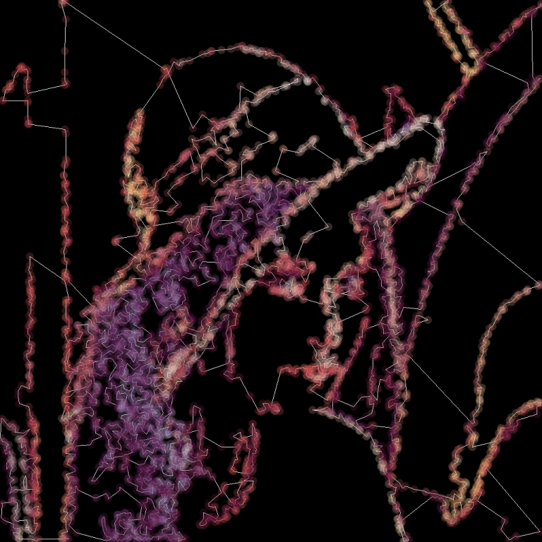
Fig. 6.3: Estimating the shortest route between hundreds of 2D points, with the G’MIC command tsp.
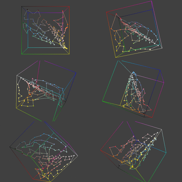
Fig. 6.4: Estimating the shortest route between several colors in the RGB cube (thus in 3D), with the G’MIC command tsp.
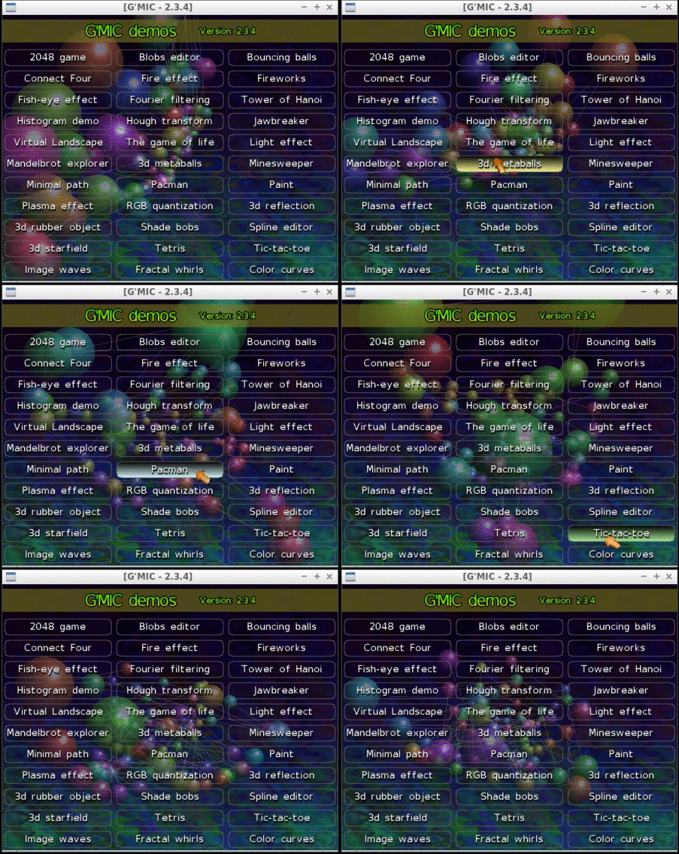
The demonstration window, which appears when gmic is run without any arguments from the command line, has been also redesigned from scratch.
Fig. 6.5: The new demonstration window of gmic, the command line interface of G’MIC.
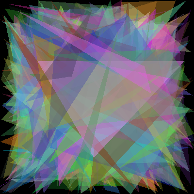
The embedded JIT compiler used for the evaluation of mathematical expressions has not been left out and was given new functions to draw polygons (function polygon()) and ellipses (function ellipse()) in images. These mathematical expressions can in fact define small programs (with local variables, user-defined functions and control flow). One can for instance easily generate synthetic images from the command line, as shown by the two examples below.
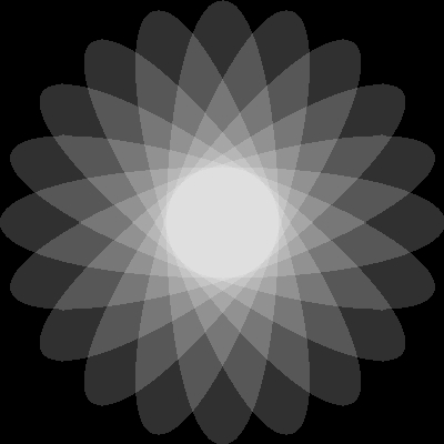
Fig. 6.7: Using the new function ellipse() from the G’MIC JIT compiler, to render a synthetic flower image.
Note also that NaN values are now better managed when doing calculus in the core, meaning G’MIC maintains coherent behavior even when it has been compiled with the optimisation -ffast-math. Thus, G’MIC can be flawlessly compiled now the maximum optimization level -Ofast supported by the compiler g++, whereas we were restricted to the use of -O3 before. The improvement in computation speed is clearly visible for some of the offered filters !
A lot of changes have also been made to the distribution channels used by the project:
First of all, the project web pages (which are now using secured https connections by default) have a new image gallery. This gallery shows both filtered image results from G’MIC and the way to reproduce them (from the command line). Note that these gallery pages are automatically generated by a dedicated G’MIC script, which ensures the displayed command syntax is correct.
Fig. 6.8: The new image gallery on the G’MIC web site.
This gallery is split into several sections, depending on the type of processing done (Artistic, Black & White, Deformations, Filtering, etc.). The last section « Code sample » is my personal favorite, as it exhibits small animations (shown as looping animated GIFs) which have been completely generated from scratch by short scripts, written in the G’MIC language. Quite a surprising use of G’MIC that shows its potential for generative art.
Fig. 6.9: Two small GIF animations generated by G’MIC_ scripts that are visible in the new image gallery._
We have also moved the main git source repository of the project to Framagit, still keeping one synchronized mirror on Github at the same place as before (to benefit from the fact that a lot of developers have already an account on Github which makes it easier for them to fork the project and write bug reports).
Voilà! Our tour of news (and the last six months of work) on the G’MIC project comes to an end.
We are happy to be celebrating 10 years with the creation and evolution of this Free Software project, and to be able to share with everyone all of these advanced image processing techniques. We hope to continue doing so for many years to come!
Note that next year, we will also be celebrating the 20th anniversary of CImg, the C++ image processing library (started in November 1999) on which the G’MIC project is based, proof that interest in free software is enduring.
As we wait for the next release of G’MIC, don’t hesitate to test the current version. Freely and creatively play with and manipulate your images to your heart’s content!
Thank you, Translators: (ChameleonScales, Pat David)

 Login
Login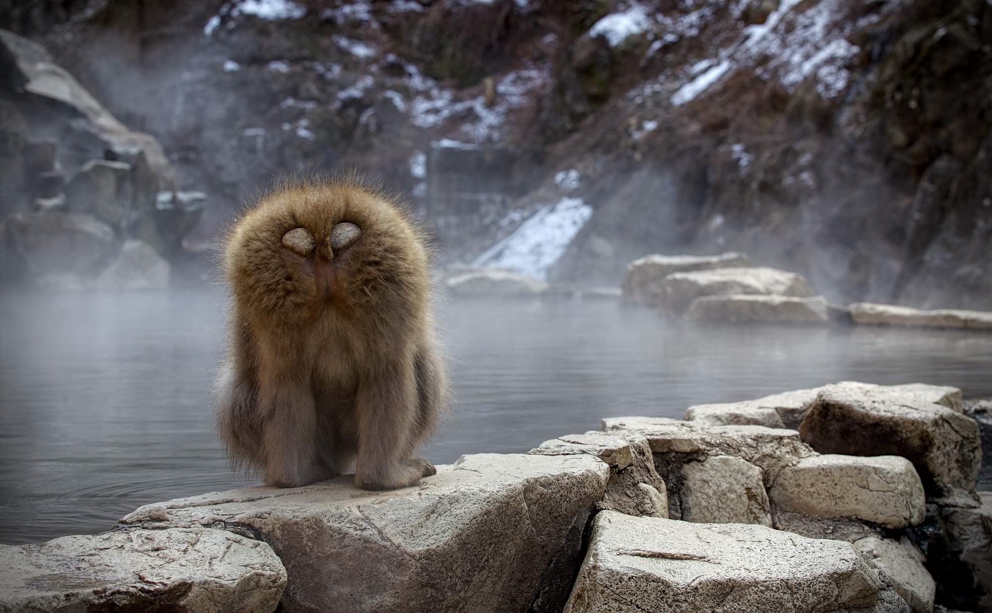





![Filter 'Mixer [PCA]'](http://gmic.eu/gmic234/fullsize/gmic_mix_pca.png)