O apresentador conversa com Mário Magalhães, autor da biografia de Carlos Marighella, recém-adaptada para o cinema, e com a atriz Maria Marighella, neta do líder revolucionário, que atua no filme e trabalha na publicação dos escritos do avô. Em seguida, a ensaísta Bianca Tavolari fala sobre a seção que passa a editar na Quatro Cinco Um, sobre a história, a vida e o futuro das cidades.
In this episode, Birgit Pauli-Haack and Mark Uraine discuss the release of Gutenberg 7.5 and 7.6 as well as WordPress 5.4, Global Styles and using Block Editor outside the editor screen — plus community contributions and WordCamp Miami. Music: Homer Gaines Editor: Sandy Reed Logo: Mark Uraine Production: Pauli Systems Show Notes / Transcript Show […]
Edmund Gordon discusses whether Hilary Mantel's final Cromwell novel lives up to its billing - and whether, at 900-odd pages, it is the right length; Muriel Zagha looks at the female gaze in French cinema, with respect to the new film Portrait of a Lady on Fire; Irina Dumitrescu talks about how to write well, and when to break the rules
Dois dias de caminhada pela cidade de São Paulo. Um total de 50 quilômetros percorridos, partindo da Zona Oeste, até a fronteira com São Caetano, na Zona Leste. Dezenas de entrevistados. Histórias surpreendentes que revelam a alma da maior cidade do país.
Pra completar, uma trilha sonora feita exclusivamente com os sons colhidos durante a caminhada.
No início do mês, faleceu o famoso crítico literário, filósofo, ensaísta, romancista e educador franco-americano George Steiner (1929-2020).
Vez ou outra, Steiner privilegiava também a nós, musicófilos, expressando a sua paixão pela música. Em 2010, à ocasião das NEXUS Conferences, no Concertgebouw de Amsterdã (sede da famosa orquestra holandesa), Steiner palestrava sobre o tema: “What’s Next for the West?” (“O Que Vem a Seguir para o Ocidente?”), e encerrou a sua apresentação com um belo discurso sobre o mistério da música. Que um dos maiores críticos literários da atualidade tenha dito que a música lhe parece superior à literatura como “força de uma possibilidade transcendente” não é coisa que Euterpe poderia ignorar e, há algum tempo, postamos uma bela montagem deste vídeo (infelizmente não mais disponível) em nossa página no Facebook.
Compartilhamos agora o vídeo original, portanto, como homenagem ao mestre, com uma tradução logo abaixo por nossa cortesia.
Música, o mistério da música. O que Nietzsche chamou tão corretamente de o mysterium tremendum. O mysterium tremendum do último ato de Tristão [e Isolda], e tantos outros casos: pode ser uma Étude de Chopin, uma frase ou mais em Mozart, que nos fala que há algo além, que paradoxalmente pertence a nós profundamente, mas que de algum modo toca em um significado universal de impossibilidade. Que não somos apenas um conjunto fisiológico eletro-químico e neural, que há mais na consciência do que fiação eletrônica. A música para mim parece, mais do que a literatura, a grande força, a esperança de uma possibilidade transcendente.
Essa é a razão pela qual é vitalmente importante que nossas crianças tenham acesso, desde a mais tenra idade, a boa música. Eu soo como um velho chato reacionário, e não me desculpo por isso, mas nada me aterroriza mais do que a exclusão de música séria das vidas de milhões de crianças pequenas: a substituição de muitas formas de música pelo horror de barulho ordenado, pelo barbarismo de barulho ordenado, a derrocada ensurdecedora de não deixar uma criança encontrar boa música, de não lhe ensinar um instrumento, se possível, de não lhe ensinar a cantar, se possível.
Houve um tempo na vida diária, no século XIX e começo do século XX na Europa, em que apresentações amadoras eram uma realização natural de pessoas educadas. Não precisava ser muito bom, não precisava ser muito grande, mas era parte de se reunir e estar em contato com aquele mysterium tremendum do transcendental. Se levarem isso embora de nós, estaremos realmente em apuros. Não acho que conseguirão. Durante os piores períodos de despotismo e tirania, pessoas podiam aprender partituras de cor. Mesmo quando a música era proibida, ela ainda podia ser confiada à memória. A música é algo muito difícil de se censurar – sim, ela pode ser interrompida, ela pode ser suprimida, músicos podem ser caçados, e perseguidos, e torturados. Mas, ainda, ela está lá, e sempre o seu estranho mistério permanece.
O Concertgebouw é um lugar para se lembrar dos últimos concertos daquele gênio muito ambíguo, [Wilhelm] Furtwängler. A luz caía regularmente e temos gravações em que você ouve o tiroteio da artilharia russa se aproximando de Berlim. Em uma gravação de Beethoven e uma de Haydn daquele tempo, tocados no escuro, as pessoas na plateia, sabendo que estavam condenadas a um destino horrível…, e não há gravações ou interpretações, que eu conheça, maiores daquela música. Há algo na música que é muito mais forte mesmo nas nossas maiores apresentações, a música em certo sentido nos toca, somos tocados por ela. Isso não significa que haverá consenso sobre os seus significados, não significa que não continuaremos debatendo ferozmente sobre a escolha de um andamento lento de uma sinfonia de Bruckner para marcar a morte do Führer. Temos uma gravação e ela também é fantástica, assim como outras gravações excelentes.
Por muitos e muitos anos, eu tentava entender por que a música não diz “não” em certas ocasiões. Dachau, como vocês sabem, fica nos arredores de Munique, muito próxima, e os trens com as pessoas morrendo dentro deles de sede e de fome a caminho para Dachau costumavam passar não muito longe da sua grande sala de concerto. Nessa sala, [Walter] Gieseking apresentava o seu ciclo de Debussy, e bons críticos dizem que nunca houve uma interpretação superior de Debussy. E a minha pergunta era, para estudantes alemães – e comecei a perguntá-la imediatamente após a Guerra –, para crianças de escolas alemãs, por que a música não disse “não”? – o que é uma pergunta sem sentido. Mas é uma pergunta sem sentido? Ainda não sei a resposta. Poderia a música ter se recusado a ser tocada? É claro que poderia. Poderia ser tocada de modo errado pelo menos? Poderia Gieseking tocar notas erradas pelo menos? Não tocou.
Então o mistério permanece, mas também permanece a forte e urgente esperança de que não deixaremos que nos levem embora essa experiência sobrepujante, esse privilégio de existir, que é a grande música.
This week the TLS is running an extract from The Mirror & the Light, the long-awaited third and final volume of Hilary Mantel’s Thomas Cromwell novels. In 1538 Thomas Cromwell, Lord Privy Seal, questions Geoffrey Pole, the youngest son of a great family. Pole is accused of conspiring against Henry VIII and attempting to bring back the old religion and reinstate the Pope as head of the Church. (The Mirror & the Light will be published on March 5 by Fourth Estate. The audio book is published by W F Howes and narrated by Ben Miles.)
James Shapiro, the author of Shakespeare in a Divided America, discusses the history of West Side Story, the most popular and successful Shakespeare musical of all time, and Ivo van Hove's flawed Broadway adaptation; Toby Lichtig reviews Tom Stoppard's new play Leopoldstadt and talks us through a selection of Jewish-focused pieces in this week's issue of the TLS; David Horspool, the TLS's history editor and a keen consumer of audiobooks, tells us what he has been listening to this month
West Side Story, directed by Ivo van Hove
Leopoldstadt by Tom Stoppard, Wyndham's Theatre, London, until June 13
O diretor de Bacurau Kleber Mendonça Filho e a psicanalista Maria Rita Kehl falam sobre cinema, psicanálise, cultura, crítica, Brasil e outros temas no primeiro bloco. Em seguida, o apresentador Paulo Werneck e o repórter Chico Felitti conversam com o poeta Ismar Tirelli Neto. Por fim, Rafael Freitas da Silva comenta sobre seu livro O Rio Antes do Rio, que inspirou o enredo da Portela em 2020.
Rebecca Langlands on lessons learnt in the only known ancient Roman brothel; Caroline Moorehead reviews Elena Ferrante's latest novel; Rory Waterman reads a new poem, "Defences" ("'Crikey!' you say. 'It’s gorgeous!'...")
Books:
The Brothel of Pompeii: Sex, class, and gender at the margins of Roman society, by Sarah Levin-Richardson
Em 1974 um bioquímico da universidade de Stanford chamado Paul Berg desenvolveu uma tecnologia que permitia inserir o DNA de um vírus de macaco numa bactéria. O vírus SV40 causava câncer em ratos de laboratório. E a bactéria em questão, a E. Coli, era uma das mais abundantes no intestino humano.
A descoberta assustou o mundo científico. E se essas bactérias mutantes escapassem para os laboratórios, de lá para o mundo e de repente a humanidade se visse às voltas com uma pandemia de câncer?
Diante disso, a comunidade científica resolveu fazer algo raro: parar tudo para pensar.
No ano seguinte, cientistas do mundo todo se reuniram na Califórnia para o evento que ficou conhecido como Conferência de Asilomar, onde foram definidas boa parte das regras que ainda hoje regem a ética da biotecnologia.
Desde então, várias outras tecnologias, igualmente impactantes, foram descobertas. Algumas delas, como a inteligência artificial, podem modificar profundamente nossas relações sociais, políticas e econômicas. Mais do que isso, podem alterar profundamente a essência da nossa espécie.
Quais são essas tecnologias? Como lidamos com ela até aqui? Que impactos reais podemos esperar nos próximos anos, décadas ou séculos? Como será o futuro se pudermos escolher as características dos nossos bebês?
Ouça de graça no seu aplicativo de podcasts predileto!
*****
– Colabore com a Rádio Escafandro e receba recompensas.
Professor livre-docente da Universidade de São Paulo, associado ao Laboratório de Microbiologia do Instituto de Ciências Biomédicas. Biólogo, possui doutorado em genética molecular pela Universidade de Tel-Aviv e pós-doutorado na Universidade de Sydney.
Jornalista especializado em ciência, colunista da Folha de S.Paulo, doutor em Ciências Sociais, autor dos livros ‘Promessas do Genoma’ e ‘Ciência: Use com Cuidado’.
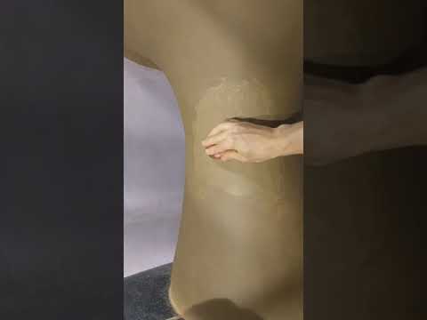
One process for burnishing fine clay plaster; this is wet burnishing, where clay is dampened first, then the creamy clay that comes to the surface is compressing into any micro-pores in the surface. This particular example is a pedestal sink that I burnished over a dozen times using this method. The result is a very smooth tight surface. The sink bowl is coated with as much hardening oil as it would absorb (I use linseed stand oil) to repel water.
Is it the best of times or the worst of times to be a satirist? Madeleine Brettingham, a writer on the BBC's News Quiz, joins us to discuss; Toby Lichtig on a new production of Endgame and the constraints imposed on Samuel Beckett adaptations; founded in the 1960s, the Oulipo was – and remains – a group of writers and scientists striving for "potential literature". Anna Aslanyan considers the movement's legacy
March of the Lemmings: Brexit in print and performance 2016–2019, by Stewart Lee
The Joke is On Us: Political comedy in (late) neoliberal times, edited by Julie A. Webber
Endgame / Rough For Theatre II, at the Old Vic theatre, London
The Oulipo and Modern Thought, by Dennis Duncan
All that is Evident is Suspect: Readings from the Oulipo 1963–2018, edited and translated by Daniel Levin Becker and Ian Monk
In this episode, Birgit Pauli-Haack and Mark Uraine discuss the release of Gutenberg 7.4 and 7.5 with more enhancements and fixes. They also cover some interesting block editing features, Community Contributions, and the upcoming release of WordPress 5.4. Music: Homer Gaines Editor: Sandy Reed Logo: Mark Uraine Production: Pauli Systems Show Notes / Transcript Show […]
No primeiro episódio de 2020, uma conversa sobre as memórias de infância do escritor japonês Haruki Murakami com a tradutora Rita Kohl e o escritor Arthur Dapieve. No segundo bloco, Marília Kodic, editora da Quatro Cinco Um, conversa com o escritor Alberto Mussa sobre os sambas do carnaval carioca 2020.
One of Germany's most acclaimed novelists talks to Maren Meinhardt about his new novel, Tyll, a vivid account of a seventeenth-century trickster's journey through a Europe ravaged by the Thirty Years’ War.
Caryl Emerson on Tolstoy’s art, ideas and life, and the extent to which these came together; Benjamin Markovits returns to a treasured childhood book: The Advanced Dungeons & Dragons Player's Handbook; Eve Babitz – a “fizzy”, “fabulous” chronicler of 1960s and 70s Los Angeles – is mid revival. Megan Marz fills us in.
Lives and Deaths: Essential stories by Leo Tolstoy, translated by Boris Dralyuk
Leo Tolstoy: A very short introduction by Liza Knapp
Leo Tolstoy by Andrei Zorin
The Advanced Dungeons and Dragons Players Handbook by Gary Gygax
I Used To Be Charming: The rest of Eve Babitz, edited by Sara J. Kramer
Hollywood’s Eve: Eve Babitz and the secret history of L.A., by Lili Anolik
Em junho de 2013, o Movimento Passe Livre (MPL) iniciou uma série de protestos, em São Paulo, contra o aumento de vinte centavos nas tarifas de ônibus e metrô.
Em pouco tempo, as manifestações ganharam uma dimensão inesperada. E mesmo depois de Estado e Prefeitura terem voltado atrás com o aumento, as ruas continuaram inflamadas por passeatas, numa ebulição popular inédita no país.
As pautas se multiplicaram. O combate à corrupção e a demanda por melhores serviços públicos no geral passaram a engrossar o coro das ruas.
Até que, no final de 2014, as cores das manifestações foram mudando. Um movimento que era essencialmente progressista ganhou ares nacionalistas, conservadores e anti-partidários.
Grupos recém-criados como o Movimento Brasil Livre (MBL) e o Movimento Vem Pra Rua, passaram cooptar essa insatisfação popular difusa que culminaria no impeachment de Dilma Roussef. E que seria um dos vários fatores que colaboraram para a eleição do governo de extrema-direita de Jair Bolsonaro.
Como isso aconteceu? Como o Passe Livre conseguiu transformar uma pauta única num protesto nacional? Como grupos de direita, notadamente o Movimento Brasil Livre (MBL) se apropriaram das manifestações? Quem financiou esses grupos? Como a direita foi capaz de canalizar o sentimento de revolta e por que a esquerda não conseguiu retomar as ruas desde então?
Ouça de graça no seu aplicativo de podcasts predileto!
*****
– Colabore com a Rádio Escafandro e receba recompensas.
Doutor em ciências da computação, professor da Escola de Artes, Ciências e Humanidades da USP (EACH-USP) e cocoordenador do Monitor do Debate Político no Meio Digital.
Lucy Dallas reports on theories, developments and disputes in the world of science fiction; Lawrence Douglas adds crucial historical context – stretching back to the Middle Ages, in fact – to the current US presidential impeachment; the poet Hannah Sullivan emerges from Princeton University Library with fresh insight into T. S. Eliot's love letters
The Carrier Bag Theory of Fiction by Ursula Le Guin
Darktable is slowly converging to a scene-referred RGB workflow. Why is that? What does it involve? How does the use of darktable change? Answers here…
This article begins with a 3 section introduction of the Lab space. You don’t need to understand it in detail in order to understand what happens next.
What is Lab?
The color space CIE Lab was published in 1976 by the International Commission on Illumination (CIE), in an attempt to mathematically describe the color perception of the average human being. Lab space aims to decouple the brightness information (L channel) from the chroma information (channels a and b) and takes into account the non-linear corrections that the human brain makes to the linear signal it receives from the retina. Lab space is derived from CIE XYZ space, which represents the physiological response of 3 of the 4 types of photo-sensitive cells in the retina (the cones).
The XYZ space represents what happens in the retina, and Lab represents what subsequently happens in the brain, but both color spaces are
models,
that is, attempts to describe reality and not the reality itself. There are always discrepancies between a model and reality, but these models are refined and improved as research progresses. Moreover, a model often represents reality only under certain conditions and assumptions, which define the area of validity of each model.
Regarding their respective areas of validity, XYZ works well almost all the time, Lab only works as long as the image has a contrast less than 100:1 (i.e. a maximum dynamic range of 6.5 EV). In the context of the creation of the Lab model in 1976, researchers were working with scanned negatives, and color negatives have a dynamic range of 6 to 7 EV. 6.5 EV is also the static contrast of the retina, and it was a little after 1976 that we realized that the brain was constantly performing HDR fusion of several images per second, meaning that static contrast as a model parameter doesn’t make much sense in the context of human vision.
What is CIE Lab for? It is intended to predict the perceptual difference between 2 colors (the delta E) and to make gamut adaptations when converting an image from one color space to another. One can then try to remap the gamut to the closest color in the target color space via strategies that minimize the delta E digitally.
The big disadvantages of Lab are:
It doesn’t work well for strong contrast (> 7 EV), and especially outside the range [1:100] Cd/m²,
It is not linear in hue, i.e. if one fixes a pixel’s a and b chromaticity components and changes only its brightness L, the same hue would be expected at a different brightness (this was the design purpose of the Lab space), however there is a slight shift in the hue, more or less marked depending on the original color of the pixel.
What is Lab doing in darktable?
The original idea was to allow separate manipulation of the brightness and chromaticity. In 2009, the year of the project’s creation, cameras had dynamic ranges quite close to Lab’s valid range; the idea was far from bad at the time, especially because darktable did not have a complex masking option then.
Advantages:
Lab, being a reference space and therefore independent of the display color, makes presets very easy to set up and transfer,
Lab sets the middle gray (18%) to 50%, so the interface is more intuitive (the middle gray is in the middle of the graph of the tones, for example).
Problems:
Today’s cameras have dynamic ranges that are largely outside of the conditions under which Lab is valid, which makes the defects of this space more apparent. With dynamic ranges from 10 to 14 EV at 100 ISO, any recent camera does HDR by default, and Lab is not designed to handle that much dynamic range
Pushing pixels in Lab space is very risky, especially when tackling compositing and image fusion with softened and feathered masks. We’ll get back to that, but it has to do with the next problem…
Lab is not adapted to physically realistic corrections, such as blurring, deblurring, denoising, and any filter that simulates or corrects for an optical effect.
In brief, Lab was a youthful mistake. That said, all other photo processing pieces of software seem to work by default in non-linear RGB spaces (with a “gamma” applied at the beginning of the pipe) that are basically equivalent (regarding their flaws and drawbacks for image filters).
How does Lab work?
Everything (e.g. the camera sensor) starts from a linear RGB space. We convert linear RGB to XYZ. For the purposes of the demonstration, we can consider the XYZ space as a special RGB space whose primary colors have been slightly manipulated (that’s not the case, but it behaves the same way). XYZ is also a linear space.
We then switch from XYZ to Lab by applying a “gamma correction” on the luminance channel (from Y to L), and a rotation on the channels a and b. Mathematically, Lab is like applying 2.44 gamma to linear RGB – it poses the same practical problem: it’s highly non-linear.
Summary
Lab doesn’t work for high-contrast images and doesn’t work well for images with moderate contrast. It encodes pixel values in a perceptual manner rather than physical one, which will pose a problem in the following. Lab was not designed for image processing, but only as a way to study human vision.
Precision: I have used the term “gamma” or “gamma correction” incorrectly here. Strictly, a gamma function is the specific (technical) electrico-optical transfer function (EOTF) of old-school CRT screens, which is a power function with an exponent between 1.8 and 2.2. Nowadays, people incorrectly name “gamma” any power function used for technical integers encoding or artistic lightness adjustments, which is confusing. Any encoding transfer function (using a power function or not) should be called OETF (Opto Electrical Transfer Function), and is used only to alleviate the limits of 8 bits integer file formats. Any artistic power-like brightness corrections should be called a tone curve. Even if the operation is the same, it does not have the same meaning and should not be applied at the same place in the graphics pipe. But ICC nomenclature continues to call “gamma” the exponent used to encode/decode RGB pixels when using integer file formats, so here we are, mixing unrelated concepts under an umbrella name just because the maths write the same. But, when communicating with people out of the industry, it’s often easier to use the incorrect name so that everyone sort-of understands, even if it carries on the confusion.
By the way, power-like OETF are completely unnecessary as long as you use floating point arithmetic and files format (32 bits TIFF, PFM, OpenEXR…).
The limits of non-linear spaces in image processing
First of all, what do we mean by “linear”? If y is linear with respect to x, it means there’s a relationship between x and y in the form y= a . x + b, where a and b are real constants. Linear means proportional to something plus or minus a constant.
So, when we talk about linear RGB space, we mean that the RGB values are proportional to something. But proportional to what?
The sensor counts the number of photons it receives at each photosite. Every pixel contains information on the light spectrum captured at its position, in the form of 3 intensities (red, green, blue). The coefficient of proportionality a between the number of photons and the final RGB value is the ISO sensitivity of the sensor. The constant b is the sensor noise threshold. The RGB signal is proportional to the energy of the light emission picked up by the camera sensor.
From the point of view of human perception, these intensities being proportional to the physical energy level of the light emission, does not make sense. In fact, the brain applies a non-linear, logarithmic correction that the Lab color space approximates using a cubic root. This means that we have an increased sensitivity to dim light, and reduced sensitivity to bright light.
However, all optical operations that are performed during image capture (e.g. lens blur, noise creation, or the effect of a color filter added to the lens) are applied directly to the photons. To reverse the lens blur or to simulate it when processing, we need to work on the linear RGB information, which is the closest thing to the photon data that is available to us.
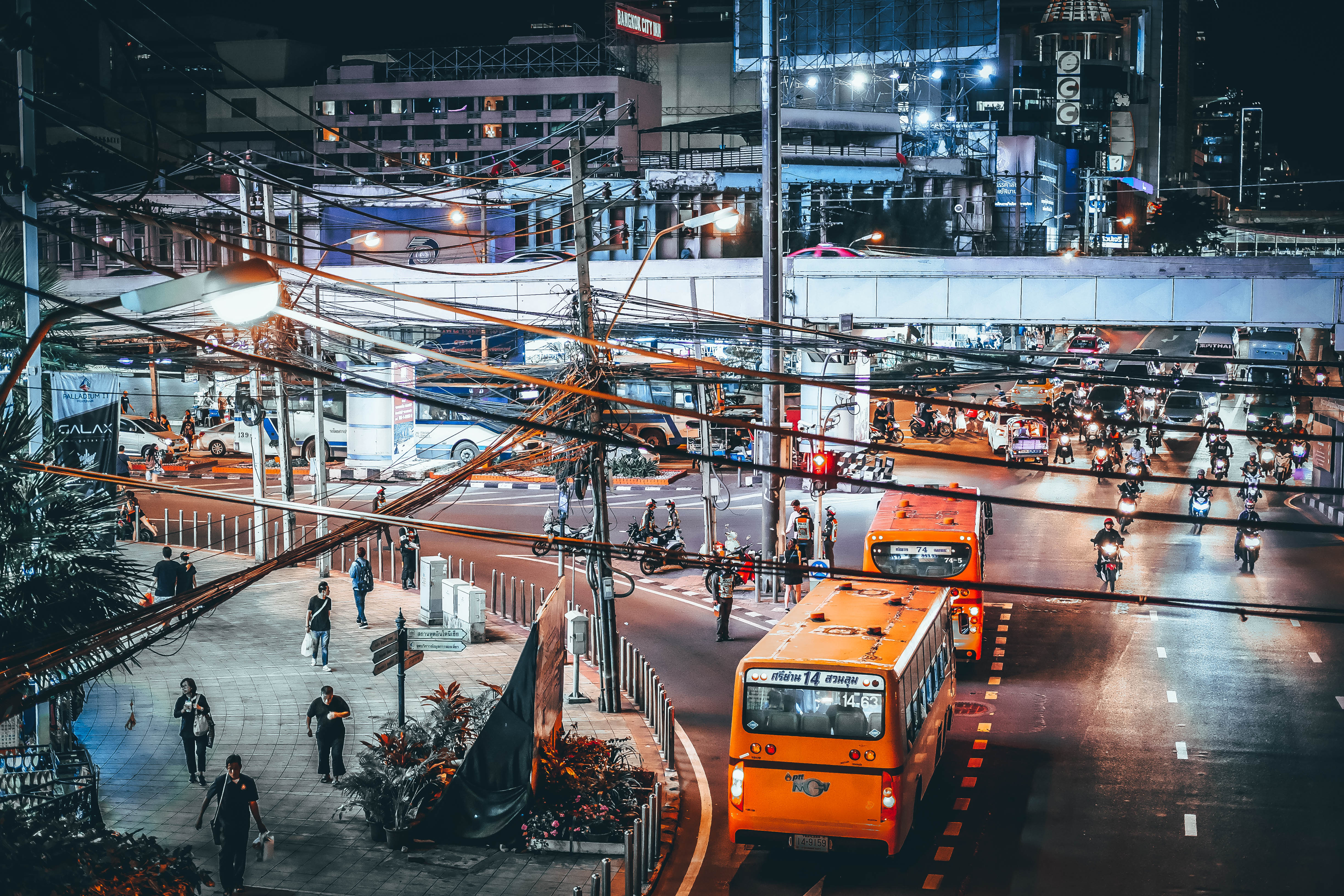
Lens blur applied in sRGB
Lens blur applied in linear RGB then encoded in sRGB
Original photo: Hanny Naibaho
Observe in particular how the dark silhouettes (bottom left) merge into the light background, or the contrast of the pentagons formed by the lens diaphragm on spotlights.
Another example, with a simple blur on smooth surfaces: Which of these gradations seems to you to be the most progressive?
Left: Linear RGB blurring sRGB encoding; Right: sRGB encoding, then blurring
These two examples were generated with Krita, which allows you to work in both linear and non-linear RGB, and has filter layers including a physically realistic lens blur.
This type of problem will occur the same way in darktable, as soon as you use the modules sharpen,high-pass,low-pass, and feathering/smoothing of drawn and/or parametric masks (which are blurs).
Blurring, deblurring, or anything else connected to optics must take place in linear RGB. There’s no mathematical model* that allows correct gradients in RGB encoded for display (with an OETF) or in Lab, due to loss of connection between pixel values and light energy.
* and just because the problems aren’t visible all the time doesn’t mean the problems aren’t always there. We can, up to a certain point, hide them with mathematical trickery (thresholds, opacity, etc.), but they will always end up coming out at the worst time. Trust me, I know exactly where to push to make it break.
This is also the problem that arises with hue zones blending in the color zones module (even if a tweak, introduced under the “smooth” process mode, attempts to hide this under the rug), which produces granular and sharp transitions.
The only darktable module that works in Lab to make a blur, and where it still works reasonably, is the local laplacian mode of the local contrast module. The price we pay for it to work is that it’s very computationally heavy and theory is like rocket science. And, even if the blur is stable, it comes with an ungracious desaturation with a hue shift to muddy grey-blue when you push the sliders a little too hard.
The benefits of a linear RGB treatment
So here’s where you say “as long as I’m not blurring my images or working only on color, I can still use Lab”.
That’s partly true, but in fact, even in those cases, working in linear RGB is simpler, with faster algorithms that can tolerate more extreme adjustments without showing annoying side-effects. Also, once again, Lab can’t support high dynamic ranges, so care must be taken to use the Lab modules after HDR tone mapping.
Strictly speaking, the only application where Lab is required is the gamut mapping, when changing color space before sending the image to a file or to the screen. And even then, since 1976, better spaces have been developed (IPT-HDR, JzAzBz) for this purpose, in HDR and with an almost perfect linearity of hues.
The current state of darktable
With the release of darktable 3.0, the default pipeline (i.e. the basic module order) has been reordered around filmic RGB. There are 4 essential steps in this pipe:
the demosaic module, which converts the raw file (which only contains the intensity of a single layer, R, G or B at each pixel site) to a picture (with complete RGB data for each pixel location),
the input color profile module, which converts the sensor’s RGB space to a standard working color space,
the filmic RGB (or the base curve) module, which translates between linear space (proportional to light energy) into non-linear (perceptually compressed) space,
the output color profile module, which converts from the standard working space to the RGB space of the screen or the image file.
Note that the base curve approach remains the one applied by default because it allows darktable to more-or-less approximate the rendering of the camera JPEG as soon as the software is opened, which seems to be the preference of many users. Nevertheless, as part of darktable 3.0, the base curve was pushed back in the pixel pipe by default, to just before the filmic RGB module, which makes it safe for the colors produced by the modules that are applied earlier. The base curve module also was provided with a color preservation mode, which produces results similar to filmic RGB. Between base curve and filmic RGB,for darktable 3.0, the difference is now only about ergonomics and on the ability to recover very low light. filmic RGB is a little more complex to understand but faster to set up (once properly understood), and is more powerful when working in deep shadows.
Modules that work in linear RGB and output in linear (thus leaving the pipeline linear after them) are:
exposure
white balance
channel mixer
tone equalizer (which is linear in parts).
The advantage of performing linear operations is that they do not affect
the chrominance of the image (because changing the luminosity leaves the
chrominance intact) and preserve the energy proportionality of the
signal. These modules must be positioned before filmic RGB or the base curve. Exposure and tone equalizer are recommended prior to
the input color profile. They can be used safely and without moderation. Note that there is a catch here on the tone equalizer,
which preserves local linearity (within the image areas),
but not the overall linearity (between zones). It corresponds to what
would happen if we walked onto the scene with a flashlight, and hand reilluminated the objects in the scene, so we still keep
the physical coherence of the signal.
Modules that work in linear RGB and carry out non-linear, but chrominance-preserving operations, (provided that the chroma preservation mode is activated) are:
RGB curves
RGB levels
The chrominance is preserved via methods that constrain the RGB ratios in and out of the module, so as to keep them identical. Note that RGB curves and RGB levels can be moved before or after filmic RGB depending on the intention, since they’re doing non-linear operations anyway. On the other hand, be careful not to use the mask feathering on modules that come later, as linearity is no longer assured and mask blurring + blending could produce unpleasant results.
Modules that work in linear RGB and carry out non-linear operations without preserving the chrominance are:
local tone mapping (we’ll get back to that)
color balance
LUT 3D
Color balance is designed to be applied to linear RGB data
that hasn’t been corrected for contrast, i.e. before filmic RGB, tone curves etc. It does not preserve the chrominance because its explicit purpose
is to adjust chrominance creatively. Similarly for LUT 3D, for which
the main goal is to emulate analog film emulsions or complex aesthetic transforms.
I remind readers here that filmic RGB is a dynamic range compressor,
from the high dynamic range of the camera to the low dynamic range of the screen. It is not a tone curve intended to apply an artistic correction, but a mapping of tones to force fit the sensor data into the
the available screen space. filmic RGB tries to protect the details as much as possible (which we assume a priori are in the middle tones) and
to keep a certain optical readability in the image.
Before filmic RGB, in the linear pipe, we still find some
modules that work in Lab but perform linear operations
that should (strictly speaking) be realized in linear RGB:
contrast equalizer
high pass
low pass
sharpen
denoise (non-local means)
These modules need to be adapted in the future to be able to work on a linear Yxy space (derived from CIE XYZ) because it is a mistake to make them work in Lab (at least, as a default). It’s a relatively easy job to do,
because Yxy breaks down the luminance (Y channel) and chrominance
(channels x and y) with a logic similar to Lab, minus the
non-linear transformation. In the meantime, you can continue to
use them, but with moderation. For the contrast equalizer,
note that it uses an edge-sensitive wavelet separation,
which makes it quite cumbersome to execute, but very effective at preventing
halos, even considering that it works in Lab.
After filmic RGB, in the non-linear pipe, are all the
other Lab modules, since they require low dynamic range. Some of these modules could also be converted to xyY and moved before filmic RGB in the future (in particular the soften, grain and fill light modules). Also note that the
vignette module was left at the end of the pipe, as before, even though it works in RGB. It’s likely it’ll be better off before
filmic RGB, or even before the input profile, but its code is
surprisingly complex for what it does, and I haven’t had the time
to unravel the imbroglio in order to understand what its working hypotheses are.
Modules not recommended
A number of modules are not recommended due to fundamental errors in
design (based on my personal opinion, which is based on my
practical and theoretical experience in image retouching), and in the
spirit of streamlining the workflow with a minimum number of steps. There is nothing stopping you from continuing to use them, especially since users regularly introduce me to new use cases that I hadn’t thought of. But the idea here is to give you the keys to the best possible result as quickly as possible with as little fuss as possible.
Local Tone Mapping
Local tone mapping internally encodes RGB values logarithmically (they are then decoded at the output, so no problem at
at this level), then applies a bilateral blur to these logarithmic values. As we saw above, theory is clear: a blur, on anything non-linear, produces halos and fringes. And as promised, the default setting range of this module is much reduced, so that users have become accustomed to
merging the output of the module with low opacity –
this is only hiding the misery.
Prefer the tone equalizer.
Global Tone Mapping
This module works in Lab color space to perform HDR compression, and if
you have followed my explanations, you will understand that this is a
contradiction in terms. In addition – and this is important – the
white value is adjusted automatically from the maximum in
the image, so the overall brightness of the image may change depending on
the size of the export, due to the smoothing effect of the setting to
scale (interpolation). To be expected: a lighter or darker JPEG
than the preview in the darkroom.
Prefer filmic RGB.
Shadows and highlights
Similarly, this module works in Lab color space to perform HDR compression and uses a Gaussian or bilateral blur to isolate highlights and shadows. In practice, it gives halos quickly as soon as you push the parameters (even if the bilateral blurring lessens the problems a little), and it even tends to add local contrast (as a secondary effect) in the highlights, giving clouds a very HDR look. In the shadows, used a little hard, colors turn blue-grey. In practice, it does not work, except for minor corrections.
Prefer the tone equalizer.
Low-pass filter
The low-pass filter is actually a simple blur. A lot of people
use it to invert the contrast, and then blend it with
overlay or soft/hard/linear light, to compress the
dynamic range. This is in fact exactly what the shadows and highlights module already does in fewer steps for the user. As
mentioned above, the low-pass module works in Lab color space, so for the
blur… Expect the worst.
Prefer the contrast equalizer for blur, or the tone equalizer
for local dynamic range compression
High-pass filter
A lot of people use the high-pass module by blending it with
overlay or soft/hard/linear light, for adding
sharpness. This is in fact exactly what the sharpen module already does. The high pass is achieved by subtracting between a blur
(low-pass) and the original image, so we have the same problem as for the
low-pass because it’s still working in Lab.
Prefer the contrast equalizer for fine sharpness, or the local contrast
for the general sharpness.
Sharpen
The sharpen module was originally intended for
sensors with an optical low-pass filter as well as the
smoothing due to demosaicing in some cases. First, as this
module works in Lab, you need to avoid pushing it so much that it produces halos. Second, the internal sharpening method
(using unsharp mask) is rather archaic and
quickly artificial, even in RGB mode. Thirdly, in view of
the sharpness of modern optics, given that many sensors no longer have low-pass filters, and that most of the photos will be exported
at a reduction ratio of at least 8:1 (24 Mpx sensors to 3 Mpx
screen), pixel-level sharpness enhancement has become
practically useless. Generally speaking, the digital photographer of the 21st century would benefit from calming down with the crisp sharpness -
it would be good for everyone.
Prefer to the contrast equalizer to deflect the optics via the
presets provided, or the local contrast for general sharpness.
Monochrome
The monochrome module works in Lab, which it uses to define a
weighted contribution of certain colours to the density of the black, in order to convert color into shades of gray. The problem is
that the interface is quite sensitive to the settings, and a small
correction can produce large changes and break the
overall contrast in a rather ungraceful way. In practice, getting a predictable result
is quite difficult and this module often results in a lot of
tedious micro-adjustment sessions.
The idea of a weighted contribution of colors to the density of black
comes from silver film, which behaves exactly the same way as this. But, as you saw coming, film doesn’t work in Lab and is not perceptually realistic. This idea is taken up in a physically realistic way in the channel mixer module, where several emulsion presets of commercial silver film are offered to create a grey channel. Note that, in order for the coefficients to be accurate, the colour space of the operating mode (in the module input profile) must be set to REC 709 linear, otherwise the settings will have to be adjusted.
For a black and white treatment that is based on human perceptual luminance
(linear), simply lower the input or output saturation to 0% in the color balance module (right-click on the slider and enter 0
on the keypad – the setting is only up to 50% by default in
the interface).
Prefer the channel mixer for a silver approach or the color balance for a perceptual approach.
Fill light/Bloom/Zone System
These three modules aim to re-illuminate a part of the image, and attempt
to dilute the correction in intensity and in space by blurring
in the picture. But since they’re working in the Lab color space …I won’t say it again… The results are just bad all the time, except
with very soft settings, in which case you didn’t’ really need those modules in the first place.
Prefer the exposure module with masks, or the tone equalizer
Color Correction
Every photograph has at least two sources of light: a
direct source (lamp, sun, candle) and a reflected source (walls,
clouds, floors, ceiling). It often happens that the white balance of
these two sources does not coincide. In practice, human vision has ways to correct for this this, but not the camera. So it requires a separate white balance correction for the highlights
(which generally receive direct light) and the shadows (which usually receive reflected light).
This is what the color correction module offers you, again in Lab color space, and with mixed and unnatural results as soon as you push the adjustment. When you think about it carefully, the white balance can be reduced to discussions of light spectrum, and the correction is simpler in RGB, especially to manage progressively of correction.
The color balance module allows you to adjust this
quickly, and not just for the shadows and the highlights, but
also for midtones. Using the color-pickers, to the right of the
tint sliders, it also allows you to go directly to sample
neutral tones in the image (for black, gray and white) and
let the software calculate the complementary color. See the manual
for more details.
Prefer color balance.
Velvia
Velvia works in RGB and works on a logic quite similar to the
color balance saturation. On the surface, it smells good. Except
that in fact, its colorimetric equation is not perceptually
correct. What it’s doing is changing the saturation
(which is its intention), but at the same time it also changes the hue and brightness (which
becomes awkward). The problem is that it seems to have been optimized for non-linear RGB. As a result, it is the kind of module that is typically unpredictable.
Prefer color balance.
Levels/RGB Levels
These two are working as they should, no problem with that. But
when you look at the code, you can see that it duplicates exactly the
slope/offset/power mode of the color balance module. The white point is scaled by a simple exposure correction, such as the
slope factor or even the exposure of the exposure module. The
black point is adjusted by adding a constant, such as the factor of
the offset, or the black level correction of the exposure module. The
grey point is adjusted by a power function (sometimes improperly called
gamma), just like the power factor of the color balance.
They are not just the same features, they are exactly the same
math. The difference is therefore not only in ergonomics, but
also in the fact that the color balance gives you the numerical value
settings, making them more easily transferable from one image to another or from one application to another.
Curves and levels also assume you work SDR images, with data encoded between 0 and 1. If you work HDR
pictures or raised the exposure quite a lot earlier in the pipe, the pixel values will not be clipped, but the GUI
will not give you control over the pixels above 1 (or 100 %).
If you already use the color balance, there is no need to add an additional level module. Finish your retouching in the same module.
Curves/RGB Curves
These also work well, but considering their classic use …
are they really useful? Usually they are used to
add/remove brightness, which falls in the same use case as the grey of the levels module or the power of the color balance module, or to add/remove contrast, which can be adjusted
or by decreasing/increasing the interval between white and black (in a
linear way) or by applying a non-linear brightness compression, again available from color balance.
Curve ergonomics is a real problem in an RGB linear workflow, because the middle gray is assumed to be in the center of the graph, which
therefore assumes that we are working in non-linear RGB (where the gray at
has been increased to 50%). In a linear encoding, the standard medium grey is
expected at 18% (but the practice depends or where you anchored your exposure in camera), and the
contrast control around this value not being centered on the graph
becomes complex in the interface. In addition, the graph of the curves
assumes a limited RGB signal between the values 0 and 100% (or 1)… 100% of
What? White screen luminance. In a linear workflow, the
HDR signal can go from 0 to infinity, and it is at filmic RGB step
that we’re in charge of putting everything back between 0 and 100% of the white screen.
The contrast in the color balance module is compatible with this approach using the contrast fulcrum parameter, which allows the selection of the
contrast reference. Thus when changing the contrast, we increase the light above the fulcrum, and reduce it below, but the fulcrum remains unchanged. The
display workflow (in Lab or non-linear RGB) always has the implicit assumption that gray is 50%, uses it as a contrast reference, and doesn’t allow you to change that value.
Prefer color balance.
Contrast/Brightness/Saturation
Module working in Lab, which duplicates again the modules
levels, curves, and color balance while adding undesirable effects on colours.
Prefer color balance.
Modules to be used with care
There is no correct replacement for the following modules for the moment, but they should be used with caution because
they can be unpredictable and can cause you to lose a lot of
time.
Vibrance
Vibrance works in Lab by applying a saturation correction that
penalizes already saturated pixels to avoid over-saturation, but
also tends to darken colors. The result is far from ugly, but
the problem is that we can’t control how much we darken for
the amount we resaturate.
Prefer color zones with a selection by saturation.
Color zones
This module would be awesome if the merging of colour zones were more
progressive. It now has two processing modes (strong,
the old, and smooth, the new) which are trying to meet this challenge of
two different ways, resulting in transitions too discrete for the
new, and too abrupt for the old. One more
time, it works in Lab, when similar functionality in
Capture One seems to be using HSL or HSV, which seems to perform better than Lab.
In some cases, color zones will benefit from being replaced by the
color balance module where parametric masking may be used to
isolate the shades you want to act on. Then the refinement
of the guided filter parametric mask should help in difficult cases. For the rest, color balance allows us to change the shade, saturation and brightness exactly the same.
Note, however, that the color balance module, although working in RGB
internally, merges the masks into Lab because this module is older than the
possibility to have 100 % RGB modules, and converts from Lab to RGB
internally. We’re still working on it…
Prefer color balance.
Vignetting
Adding a vignette around an image is not complicated: you just have to
to gradually lower the exposure, and eventually the saturation with a drawn mask.
However, the vignetting module performs incomprehensible black magic, which is much more complicated than that, with an
internal homogenization which would be superfluous if things were
well done. The result is rarely natural, the transition in luminosity being too violent compared to a real vignette.
You will get better results with an instance of the exposure module
set to -0.5 EV, a circular mask with a large transition area
whose polarity is reversed, possibly coupled with a desaturation in color balance to which you pass the same mask as used in exposure (via a rasterized mask).
Prefer the exposure (and, optionally, the color balance saturation) modules.
Mask blend modes not recommended.
Few people know this, but the blend modes lighten, darken,
overlay, soft light, hard light, pin light and linear light
implicitly expect the grey level to be 50% grey and are thus
totally connected to the display-referred workflow. The blend modes are going to treat
the pixels differently depending on whether they are above or below 50 %. Remember that the linear RGB workflow keeps the gray point at 18% (or even less). These blend modes will therefore behave in a way that is unpredictable in the scene-linear portions of the pipe.
In linear RGB, you should only use blend modes based on
arithmetic operations (addition, multiplication, division,
subtraction, average), on maximum/minimum comparisons
(screen) or on channel separations (hue, color, chroma, etc.).
Note that the multiply mode is one of the most powerful in linear RGB.
For example, to enhance the contrast of an image in a natural way,
it is enough to use an instance of the exposure module blended with multiply. Set the exposure between 2 and 3 EV and the opacity between 10% and 50%. Exposure is then used to control the pivot of contrast, and opacity the intensity of the effect. It’s fast, simple and effective.
A minimal workflow for beginners
In darktable, you can choose between many modules that allow you to do the same thing in a lot of different ways. But this is merely an illusion of choice, as many of them have more disadvantages than advantages (provided you want to achieve predictable results for demanding edits). If you open the code for any of the modules not recommended above, you will see that they are almost all dated 2010-2011 - the only reason we retained them was to maintain compatibility with edits performed in prior versions of darktable.
You can perform at least 80% of your processing with just 4
modules :
exposure
white balance
color balance
filmic RGB
The reason they’re so powerful is because they’re actually extremely simple, when you look at their equations:
Exposure: RGB_output = exposure × RGB_input + black level
filmic RGB is a little more complex, but it’s still high-school level math
With these 4 modules, you have everything you need to produce a correct image in terms of colorimetry, contrast, and artistic intent. Remember to turn off the base curve if you use the filmic RGB module. Then, if needed, finalize your edit with the following modules:
To improve sharpness, the best option is the local contrast module in local laplacian mode
To deblur the lens, you have deblur presets, more or less pronounced in the contrast equalizer
To denoise, the best algorithm is in the denoise (profiled) module. Use non-local means auto mode if you don’t want to break your head
To remove haze, you have haze removal
To convert to black and white, the easiest way is to use the
film presets in the channel mixer
For creative control of overall contrast and re-lighting of the scene
a posteriori, use the tone equalizer module
Some of the following modules have an underestimated power, and they are vastly underutilized:
The exposure module, with its masks, can replace all the
the other methods of mapping HDR, shadows and highlights
the tone equalizer, and even the tone curve and the local contrast (to some extent, when used with blend mode multiply)
The channel mixer module can overcome all your
gamut problems, including problems with blue in stage lighting, without having to use a fake input profile, but
also turn grass into snow or summer trees into fall trees
The color balance module can allow you to emulate the colors
of a film, compensate for uneven white balance,
remove redness on the skin, accentuate the depth and shape, create
a split-toning effect, or to give an apocalyptic atmosphere to your
images
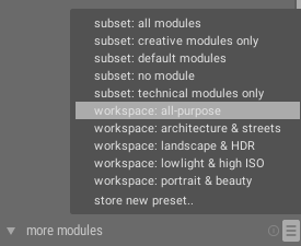
Finally, to display only a minimal selection in the interface and
modules, to the right of “More modules“, open the
list of presets and select “workspace: all-purpose“.
darktable is a lot simpler when you understand
that you don’t have to use all 77 of its modules at once …
If you have any doubts about the order of the modules, you should know that the default order for version 3.0 has been considered globally, and, apart from some uncertainties on the best position of the vignetting and monochrome modules, the rest is pretty solid, in theory and practice.
Conclusion
Pushing pixel values in either direction is one thing. Merging the corrections so they blend seamlessly together on the whole is another. We’ve seen that Lab or non-linear RGB allow the pixels to be pushed more or less
correctly, but that it is always when doing mask blending (aka occlusion) and feathering (aka blurs) that we’re paying the price. It turns out there are a lot of blurs under the hood of darktable, sometimes where you don’t expect them. It’s especially problematic when you’re compositing,
e.g. inlaying one image within another, to exchange
their background without touching the foreground. And it’s
precisely this kind of manipulation that led the movie industry
to migrate to a scene-referred linear workflow about twenty years ago.
So darktable is in transition. It’s long, it’s sometimes painful,
there are a lot of little bits to change in different places along with
grumbling users who are hungry for consistency. At least now you
know the why and the how. You also know what you have to win. I hope this helps you move forward.
For new users, limit yourself to the above recommended modules, and venture further when you begin to be comfortable. For older users, the new modules have a lot to offer to you, but old Lab modules are still relevant for
moderate creative effects and when used with knowledge of their dangers.
The linear toolbox is being expanded. On the agenda:
rewriting the 100% RGB color balance (including the
blending), with the addition of vibrance (and a vibrance equation
home-developed to preserve the color)
conversion of the contrast equalizer and soften modules to
the linear xyY space (because in fact, the Orton effect, on which the soften module is based,
is very useful when it works correctly)
a color equalizer, similar to the tone equalizer, which will allow you to adjust saturation, vibrance and Abney effect according to the pixel luminance, to pep up the filmic RGB curve
a brand-new lens deconvolution module, respectful of the depth of field (but for that, I need to develop a special wavelet based on the guided filter), which should turn your soft 18-55 mm into a Zeiss for much less
and of course the OpenCL version of the tone equalizer
There is more work than people to do it, so
wish us good luck, don’t forget to support us, and Happy New Year 2020 to all of you!
Portrait photographer in Nancy-Metz. Calculation specialist, modeling and numerical simulation for image processing (denoising, deblurring, colour management) and thermal engineering. Developer of filmic RGB, tone equalizer, color balance, and the new themeable interface for darktable 3.0. darktable user since 2010. darktable is my job, so help me out to develop.

 Login
Login